Lasers and Fabry Perots - Homework 02 Professor Craig Cahillane February 2, 2025
This is the second homework assignment for Lasers and Optomechanics at Syracuse University.
It is due Monday, February 16, 2026
You will need to complete the questions in this jupyter notebook and submit it via gitlab
Readings
Chapter 1 of Lasers by Seigman: Free eBook
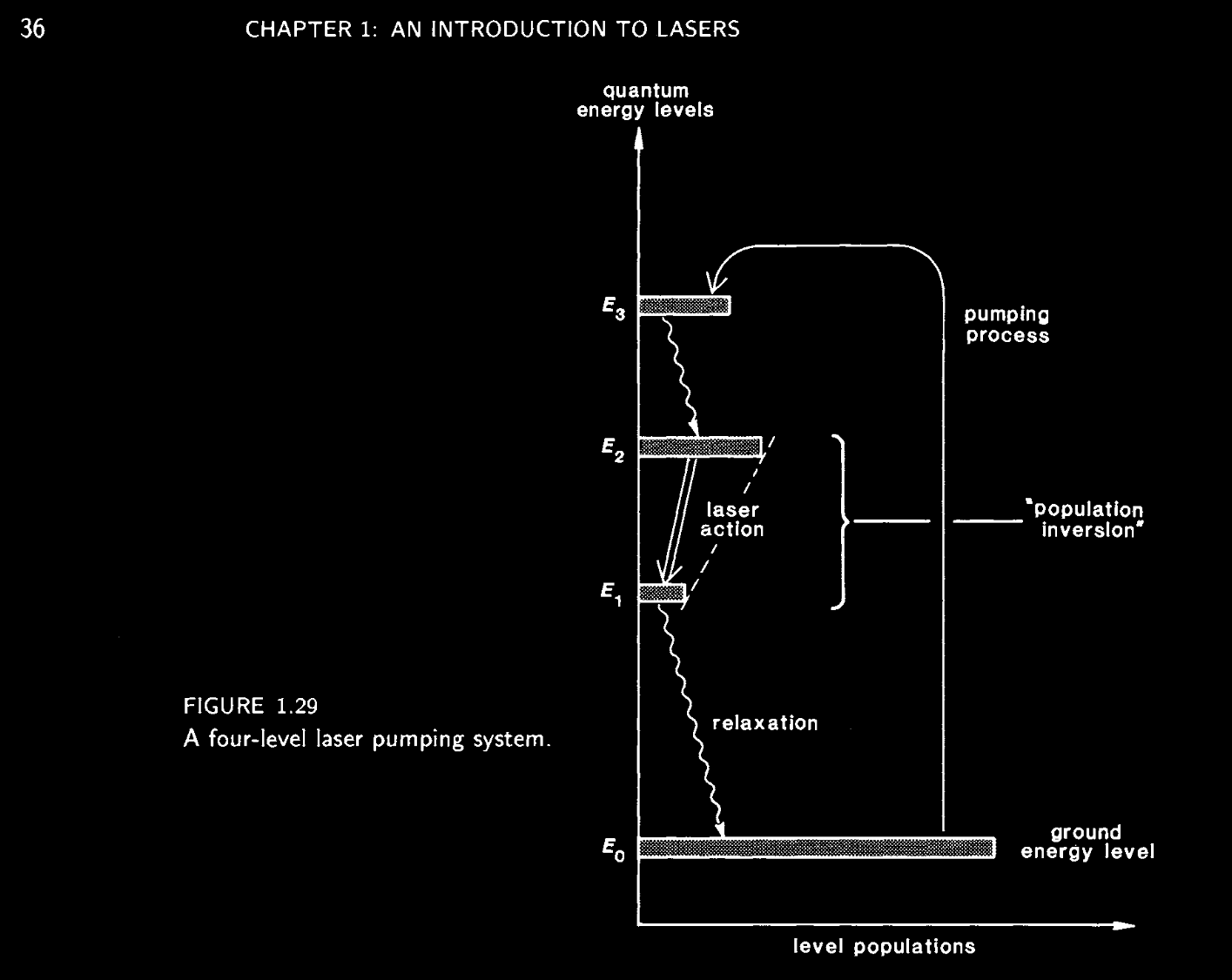
1 Atomic Rate Equations ¶ Problem 1 from Chapter 1.5 of Lasers by Siegman
1.1 Atomic Rate Equation Solution ¶ From Siegman Chapter 1.5:
d N 2 d t ≈ R p − γ 21 N 2 d N 1 d t = γ 21 N 2 − γ 10 N 1 \begin{align}
\dfrac{d N_2}{dt} \approx R_p - \gamma_{21} N_2\\
\dfrac{d N_1}{dt} = \gamma_{21} N_2 - \gamma_{10} N_1
\end{align} d t d N 2 ≈ R p − γ 21 N 2 d t d N 1 = γ 21 N 2 − γ 10 N 1 where N 1 N_1 N 1 N 2 N_2 N 2 E 1 E_1 E 1 E 2 E_2 E 2 γ i j \gamma_{ij} γ ij E i E_i E i E j E_j E j R p R_p R p E 3 E_3 E 3 E 2 E_2 E 2
Now, we add the relaxation γ 20 \gamma_{20} γ 20 E 2 E_2 E 2 E 0 E_0 E 0
d N 2 d t ≈ R p − ( γ 21 + γ 20 ) N 2 \begin{align}
\dfrac{d N_2}{dt} \approx R_p - (\gamma_{21} + \gamma_{20}) N_2
\end{align} d t d N 2 ≈ R p − ( γ 21 + γ 20 ) N 2 The d N 1 d t \dfrac{d N_1}{dt} d t d N 1
In the steady state, d N i d t = 0 \dfrac{dN_i}{dt} = 0 d t d N i = 0
0 = R p − ( γ 21 + γ 20 ) N 2 N 2 = R p γ 21 + γ 20 N 1 = γ 21 γ 10 N 2 \begin{align}
0 &= R_p - (\gamma_{21} + \gamma_{20}) N_2\\
N_2 &= \dfrac{R_p}{\gamma_{21} + \gamma_{20}}\\
~\\
N_1 &= \dfrac{\gamma_{21}}{\gamma_{10}} N_2
\end{align} 0 N 2 N 1 = R p − ( γ 21 + γ 20 ) N 2 = γ 21 + γ 20 R p = γ 10 γ 21 N 2 Population inversion requires N 2 − N 1 > 0 N_2 - N_1 > 0 N 2 − N 1 > 0
N 2 − N 1 > 0 N 2 ( 1 − γ 21 γ 10 ) > 0 R p γ 21 + γ 20 ( 1 − γ 21 γ 10 ) > 0 \begin{align}
N_2 - N_1 > 0\\
N_2 \left(1 - \dfrac{\gamma_{21}}{\gamma_{10}} \right) > 0\\
\dfrac{R_p}{\gamma_{21} + \gamma_{20}} \left(1 - \dfrac{\gamma_{21}}{\gamma_{10}} \right) > 0\\
\end{align} N 2 − N 1 > 0 N 2 ( 1 − γ 10 γ 21 ) > 0 γ 21 + γ 20 R p ( 1 − γ 10 γ 21 ) > 0 The population inversion requirement can only be satisfied if γ 10 > γ 21 \gamma_{10} > \gamma_{21} γ 10 > γ 21 E 2 E_2 E 2 E 0 E_0 E 0 no effect on the population inversion condition.
This loosely makes sense:
while it is true that N 2 N_2 N 2 γ 20 \gamma_{20} γ 20 N 1 N_1 N 1
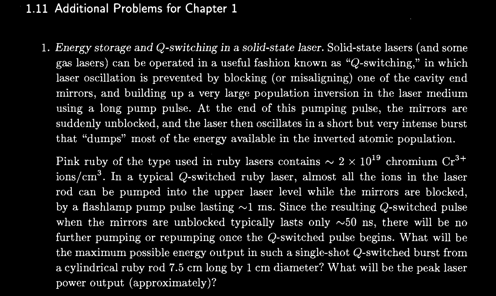
2 Pulsed Laser Power ¶ Pulsed Laser Intensity ¶ 2.1 Pulsed Laser Power + Pulsed Laser Intensity Solution ¶ Parameters:
Density ρ = 2 × 1 0 19 i o n s c m 3 \rho = 2 \times 10^{19} \mathrm{\dfrac{ions}{cm^3}} ρ = 2 × 1 0 19 c m 3 ions τ = 50 n s \tau = 50~\mathrm{ns} τ = 50 ns L m = 7.5 c m L_m = 7.5~\mathrm{cm} L m = 7.5 cm R m = 0.5 c m R_m = 0.5~\mathrm{cm} R m = 0.5 cm λ r u b y = 694.3 n m \lambda_\mathrm{ruby} = 694.3~\mathrm{nm} λ ruby = 694.3 nm
Gain Medium Volume V = π L R 2 V = \pi L R^2 V = π L R 2 N = ρ V N = \rho V N = ρ V
If all the ions discharge a photon with energy E r u b y = h ν r u b y E_\mathrm{ruby} = h \nu_\mathrm{ruby} E ruby = h ν ruby
E t o t a l = N h ν r u b y = N h c λ r u b y = ρ V h c λ r u b y = ρ π L R 2 h c λ r u b y E_\mathrm{total} = N h \nu_\mathrm{ruby} = N \dfrac{h c}{\lambda_\mathrm{ruby}} = \rho V \dfrac{h c}{\lambda_\mathrm{ruby}} = \rho \pi L R^2 \dfrac{h c}{\lambda_\mathrm{ruby}} E total = N h ν ruby = N λ ruby h c = ρ V λ ruby h c = ρ π L R 2 λ ruby h c The peak power in that pulse, assuming a flat-top pulse with equal power over the entire 50 n s 50~\mathrm{ns} 50 ns
P p e a k , f l a t − t o p = E t o t a l t p u l s e = ρ π L R 2 h c λ r u b y t p u l s e P_\mathrm{peak,flat-top} = \dfrac{E_\mathrm{total}}{t_\mathrm{pulse}} = \rho \pi L R^2 \dfrac{h c}{\lambda_\mathrm{ruby} t_\mathrm{pulse}} P peak , flat − top = t pulse E total = ρ π L R 2 λ ruby t pulse h c The peak power in the pulse for a Gaussian pulse profile will be a factor of two higher:
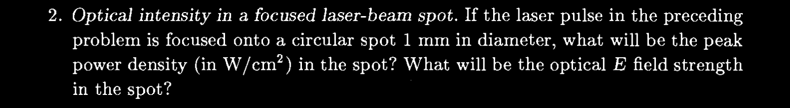
P p e a k , g a u s s i a n = 2 E t o t a l t p u l s e = 2 ρ π L R 2 h c λ r u b y t p u l s e P_\mathrm{peak,gaussian} = \dfrac{2 E_\mathrm{total}}{t_\mathrm{pulse}} = 2\rho \pi L R^2 \dfrac{h c}{\lambda_\mathrm{ruby} t_\mathrm{pulse}} P peak , gaussian = t pulse 2 E total = 2 ρ π L R 2 λ ruby t pulse h c Intensity ¶ Laser beam radius w = 0.5 m m w = 0.5~\mathrm{mm} w = 0.5 mm
For a beam radius w w w
I p e a k = 2 P π w 2 W m 2 I_\mathrm{peak} = \dfrac{2 P}{\pi w^2}~\mathrm{\dfrac{W}{m^2}} I peak = π w 2 2 P m 2 W The peak optical field strength at that spot will be
∣ E ∣ p e a k = 2 I c ϵ 0 |E|_\mathrm{peak} = \sqrt{\dfrac{2 I}{c \epsilon_0}} ∣ E ∣ peak = c ϵ 0 2 I which comes from our intensity relationship in Lecture 2:
I = 1 2 c ϵ 0 ∣ E ∣ 2 I = \dfrac{1}{2} c \epsilon_0 |E|^2 I = 2 1 c ϵ 0 ∣ E ∣ 2 import numpy as np
import scipy.constants as scc
rho = 2e19 # ions/cm^3
lambda_ruby = 694.3e-9 # m
gain_medium_length = 7.5 # cm
gain_medium_radius = 0.5 # cm
t_pulse = 50e-9 # seconds
w_beam_radius = 0.5e-3 # m

volume = np.pi * gain_medium_length * gain_medium_radius**2
NN = rho * volume

total_energy = NN * scc.h * scc.c / lambda_ruby
peak_power_flat = total_energy / t_pulse
peak_power_gaussian = 2 * total_energy / t_pulse
peak_intensity_gaussian = 2 * peak_power_gaussian / (np.pi * w_beam_radius**2)
optical_field_strength_gaussian = np.sqrt(2 * peak_intensity_gaussian / (scc.c * scc.epsilon_0))


print(f"Total Energy          = {total_energy:.1f} J")
print(f"Peak Power (Flat Top) = {peak_power_flat*1e-9:.2f} GW")
print(f"Peak Power (Gaussian) = {peak_power_gaussian*1e-9:.2f} GW")
print()
print(f"Peak Intensity (Gaussian)   = {peak_intensity_gaussian*1e-9:.2f} GW/m^2")
print(f"Peak Optical Field Strength = {optical_field_strength_gaussian*1e-9:.1f} GV/m")
Total Energy = 33.7 J
Peak Power (Flat Top) = 0.67 GW
Peak Power (Gaussian) = 1.35 GW
Peak Intensity (Gaussian) = 3433292.57 GW/m^2
Peak Optical Field Strength = 1.6 GV/m
3 Geometric Series Fabry-Perot ¶ 3.1 Part A: ¶ Rederive the Fabry-Perot intracavity electric field E c a v E_\mathrm{cav} E cav
∑ n = 0 ∞ x n = 1 + x + x 2 + ⋯ x n + ⋯ = 1 1 − x iff ∣ x ∣ < 1 \begin{align}
\sum_{n=0}^\infty x^n = 1 + x + x^2 + \cdots x^n + \cdots = \dfrac{1}{1 - x} \qquad \text{iff} |x| < 1
\end{align} n = 0 ∑ ∞ x n = 1 + x + x 2 + ⋯ x n + ⋯ = 1 − x 1 iff ∣ x ∣ < 1 Hint 1: Set up some contributing fields E n E_n E n n n n
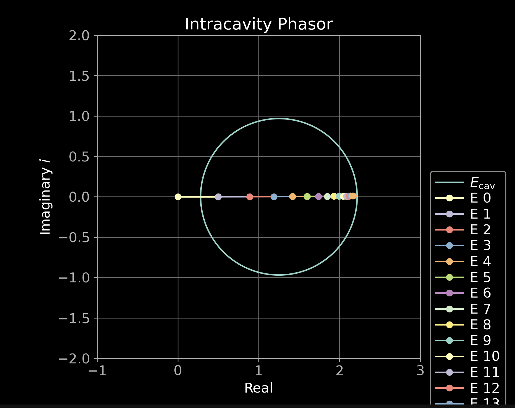
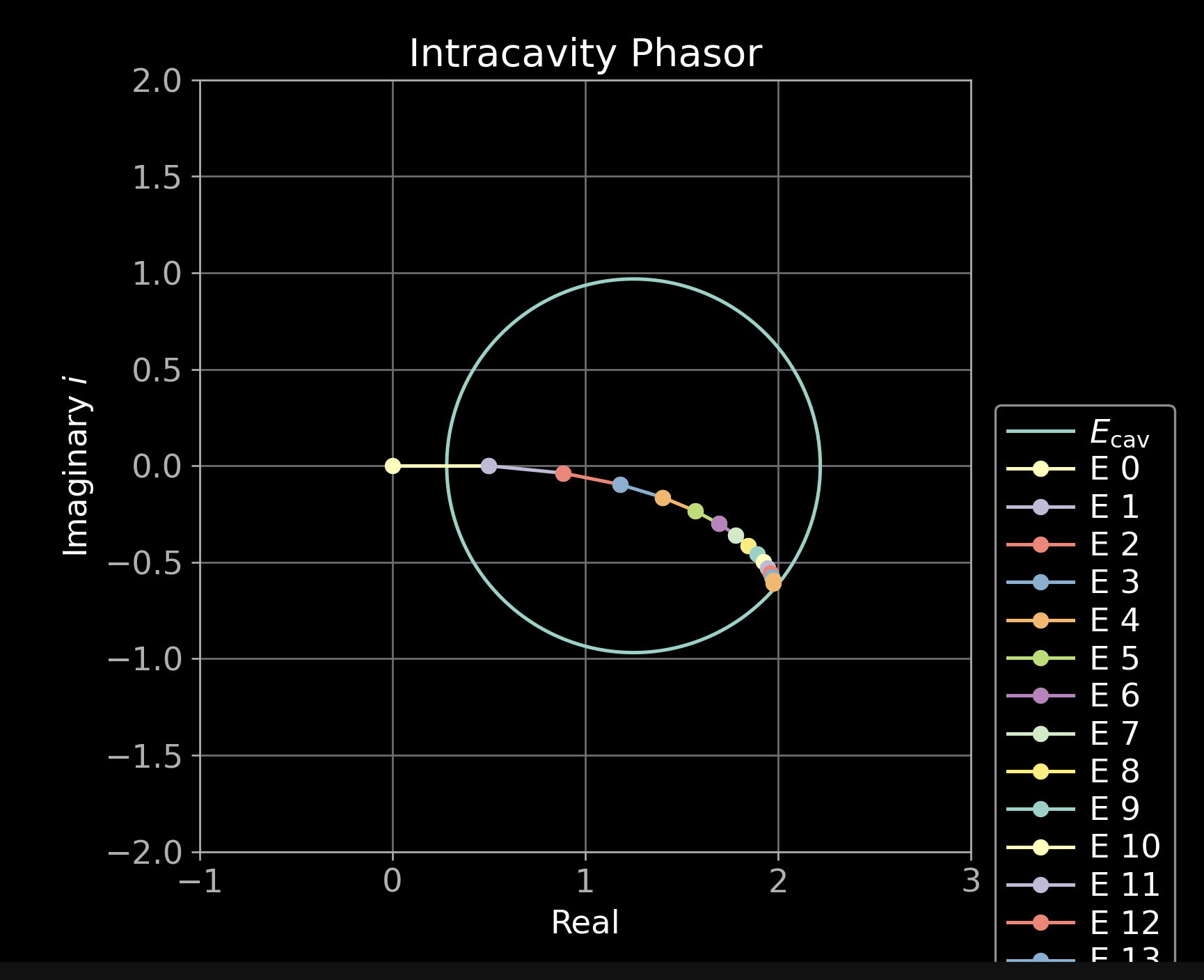
3.2 Part B: ¶ Draw a plot of the first couple of electric fields E n E_n E n E c a v E_\mathrm{cav} E cav
while on resonance,
while just off resonance, ϕ r t ≠ 0 \phi_\mathrm{rt} \neq 0 ϕ rt = 0 ϕ r t ≪ 1 \phi_\mathrm{rt} \ll 1 ϕ rt ≪ 1
3.3 Part C: ¶ The previous parts we’ve assumed there is zero delay in the propogation time: i.e that the fields in the cavity are in steady state .
Now let’s relax this assumption.
What will be the response of the Fabry-Perot intracavity field E c a v E_\mathrm{cav} E cav E i n E_\mathrm{in} E in ?
For simplicity, assume that the input laser is exactly on resonance, such that e i 2 k L = 1 e^{i 2 k L} = 1 e i 2 k L = 1
What is the round-trip time delay time τ r t \tau_{rt} τ r t
How much time t t t n n n E n E_n E n n n n t t t τ r t \tau_{rt} τ r t
Using a partial geometric series, what is the buildup for the cavity E c a v ( n ) E_\mathrm{cav}(n) E cav ( n ) n n n
Using the model 1 − exp ( − t / τ s t o r a g e ) 1 - \exp(-t / \tau_\mathrm{storage}) 1 − exp ( − t / τ storage ) τ s t o r a g e \tau_\mathrm{storage} τ storage
Compare your result to the cavity pole ν p \nu_p ν p
3.4 Geometric Series FP Solution ¶ Part A: ¶ As stated in class,
we want to have the sum from n ∈ [ 0 , ∞ ) n \in [0, \infty) n ∈ [ 0 , ∞ )
E n = t 1 ( r 1 r 2 e 2 i k L ) n E i n E_n = t_1 (r_1 r_2 e^{2 i k L})^n E_in E n = t 1 ( r 1 r 2 e 2 ik L ) n E i n Let x = r 1 r 2 e 2 i k L x = r_1 r_2 e^{2 i k L} x = r 1 r 2 e 2 ik L a = t 1 E i n a = t_1 E_in a = t 1 E i n r 1 r 2 < 1 r_1 r_2 < 1 r 1 r 2 < 1
E c a v = t 1 1 − r 1 r 2 e 2 i k L E i n E_\mathrm{cav} = \dfrac{t_1}{1 - r_1 r_2 e^{2 i k L}} E_\mathrm{in} E cav = 1 − r 1 r 2 e 2 ik L t 1 E in Part B: ¶ On resonance:
Slightly off resonance:
Part C: ¶ Exactly on resonance, we have
E c a v = t 1 1 − r 1 r 2 E i n E_\mathrm{cav} = \dfrac{t_1}{1 - r_1 r_2} E_\mathrm{in} E cav = 1 − r 1 r 2 t 1 E in The round-trip delay time τ r t = 1 F S R = 2 L c \tau_{rt} = \dfrac{1}{\mathrm{FSR}} = \dfrac{2 L}{c} τ r t = FSR 1 = c 2 L
E n E_n E n n n n t = n τ r t t = n \tau_{rt} t = n τ r t n n n n = t τ r t n = \dfrac{t}{\tau_{rt}} n = τ r t t
The partial geometric series is
a ∑ i = 0 n − 1 x i = a 1 − x n 1 − x a \sum_{i=0}^{n-1} x^i = a \dfrac{1 - x^{n} }{1 - x} a i = 0 ∑ n − 1 x i = a 1 − x 1 − x n using our definitions of x x x a a a
E c a v ( n ) = t 1 E i n ∑ i = 0 n − 1 ( r 1 r 2 e 2 i k L ) i = t 1 E i n 1 − ( r 1 r 2 e 2 i k L ) n 1 − r 1 r 2 e 2 i k L E_\mathrm{cav}(n) = t_1 E_\mathrm{in} \sum_{i=0}^{n-1} (r_1 r_2 e^{2 i k L})^i = t_1 E_\mathrm{in} \dfrac{1 - (r_1 r_2 e^{2 i k L})^n}{1 - r_1 r_2 e^{2 i k L}} E cav ( n ) = t 1 E in i = 0 ∑ n − 1 ( r 1 r 2 e 2 ik L ) i = t 1 E in 1 − r 1 r 2 e 2 ik L 1 − ( r 1 r 2 e 2 ik L ) n A model like 1 − exp ( − t τ s t o r a g e ) 1 - \exp\left(-\dfrac{t}{\tau_\mathrm{storage}}\right) 1 − exp ( − τ storage t )
t 1 E i n 1 − ( r 1 r 2 e 2 i k L ) n 1 − r 1 r 2 e 2 i k L = E c a v ( 0 ) ( 1 − exp ( − t τ s t o r a g e ) ) \begin{align}
t_1 E_\mathrm{in} \dfrac{1 - (r_1 r_2 e^{2 i k L})^n}{1 - r_1 r_2 e^{2 i k L}} = E_\mathrm{cav}(0) \left(1 - \exp\left(-\dfrac{t}{\tau_\mathrm{storage}}\right) \right)
\end{align} t 1 E in 1 − r 1 r 2 e 2 ik L 1 − ( r 1 r 2 e 2 ik L ) n = E cav ( 0 ) ( 1 − exp ( − τ storage t ) ) Recalling that the maximum steady state on resonance for the intracavity power E c a v ( 0 ) = t 1 E i n 1 − r 1 r 2 E_\mathrm{cav}(0) = \dfrac{t_1 E_\mathrm{in}}{1 - r_1 r_2} E cav ( 0 ) = 1 − r 1 r 2 t 1 E in e 2 i k L = 1 e^{2 i k L} = 1 e 2 ik L = 1 n = t τ r t n = \dfrac{t}{\tau_{rt}} n = τ r t t
t 1 E i n 1 − ( r 1 r 2 ) n 1 − r 1 r 2 = t 1 E i n 1 − r 1 r 2 ( 1 − exp ( − t τ s t o r a g e ) ) 1 − ( r 1 r 2 ) n = 1 − exp ( − t τ s t o r a g e ) ( r 1 r 2 ) t τ r t = exp ( − t τ s t o r a g e ) log ( ( r 1 r 2 ) t τ r t ) = − t τ s t o r a g e t τ r t log ( r 1 r 2 ) = − t τ s t o r a g e → τ s t o r a g e = τ r t log ( 1 r 1 r 2 ) \begin{align}
t_1 E_\mathrm{in} \dfrac{1 - (r_1 r_2)^n}{1 - r_1 r_2} &= \dfrac{t_1 E_\mathrm{in}}{1 - r_1 r_2} \left(1 - \exp\left(-\dfrac{t}{\tau_\mathrm{storage}}\right) \right)\\
1 - (r_1 r_2)^n &= 1 - \exp\left(-\dfrac{t}{\tau_\mathrm{storage}}\right)\\
(r_1 r_2)^{\frac{t}{\tau_{rt}}} &= \exp\left(-\dfrac{t}{\tau_\mathrm{storage}}\right)\\
\log\left( (r_1 r_2)^{\frac{t}{\tau_{rt}}} \right) &= -\dfrac{t}{\tau_\mathrm{storage}}\\
\dfrac{t}{\tau_{rt}} \log\left( r_1 r_2 \right) &= -\dfrac{t}{\tau_\mathrm{storage}}\\~\\
\rightarrow \tau_\mathrm{storage} &= \dfrac{ \tau_{rt} }{ \log\left( \dfrac{1}{r_1 r_2} \right) }
\end{align} t 1 E in 1 − r 1 r 2 1 − ( r 1 r 2 ) n 1 − ( r 1 r 2 ) n ( r 1 r 2 ) τ r t t log ( ( r 1 r 2 ) τ r t t ) τ r t t log ( r 1 r 2 ) → τ storage = 1 − r 1 r 2 t 1 E in ( 1 − exp ( − τ storage t ) ) = 1 − exp ( − τ storage t ) = exp ( − τ storage t ) = − τ storage t = − τ storage t = log ( r 1 r 2 1 ) τ r t From class, the Fabry-Perot cavity pole ν p = 1 2 π c 2 L log ( 1 r 1 r 2 ) \nu_p = \dfrac{1}{2\pi} \dfrac{c}{2 L} \log\left(\dfrac{1}{r_1 r_2}\right) ν p = 2 π 1 2 L c log ( r 1 r 2 1 )
Since F S R = c 2 L = 1 τ r t \mathrm{FSR} = \dfrac{c}{2 L} = \dfrac{1}{\tau_{rt}} FSR = 2 L c = τ r t 1
τ s t o r a g e = 2 π ν p \tau_\mathrm{storage} = \dfrac{2 \pi}{\nu_p} τ storage = ν p 2 π 4 Finesse and Loss in a Fabry-Perot ¶ A very convenient relationship between total loss in a cavity L t o t a l \mathcal{L}_\mathrm{total} L total F \mathcal{F} F F ≫ 1 \mathcal{F} \gg 1 F ≫ 1
F = 2 π L t o t a l \begin{align}
\mathcal{F} = \dfrac{2 \pi}{\mathcal{L}_\mathrm{total}}
\end{align} F = L total 2 π Derive this result starting with F = F S R ν F W H M \mathcal{F} = \dfrac{\mathrm{FSR}}{\nu_\mathrm{FWHM}} F = ν FWHM FSR
Hint 1: Total loss includes transmission losses for both mirrors: L t o t a l = T 1 + T 2 + L 1 + L 2 \mathcal{L}_\mathrm{total} = T_1 + T_2 + \mathcal{L}_1 + \mathcal{L}_2 L total = T 1 + T 2 + L 1 + L 2
Hint 2: Write r = 1 − T − L r = \sqrt{1 - T - \mathcal{L}} r = 1 − T − L
Hint 3: Use the binomial approximation.
Hint 4: This paper from MIT may be helpful: Loss in long-storage-time optical cavities
4.1 Finesse and Loss in FP Solution ¶ Because we are in the high finesse limit, the reflectivity of the mirrors r i r_i r i 1 − r 1 r 2 ≪ 1 1 - r_1 r_2 \ll 1 1 − r 1 r 2 ≪ 1
F = F S R ν F W H M F = c 2 L c L π arcsin ( 1 − r 1 r 2 2 r 1 r 2 ) F = π 2 1 ( 1 − r 1 r 2 2 r 1 r 2 ) F = π r 1 r 2 1 − r 1 r 2 \begin{align}
\mathcal{F} &= \dfrac{\mathrm{FSR}}{\nu_\mathrm{FWHM}}\\
\mathcal{F} &= \dfrac{\dfrac{c}{2 L}}{\dfrac{c}{L \pi} \arcsin\left( \dfrac{1 - r_1 r_2}{2 \sqrt{r_1 r_2} } \right)}\\
\mathcal{F} &= \dfrac{\pi}{2} \dfrac{1}{\left( \dfrac{1 - r_1 r_2}{2 \sqrt{r_1 r_2} } \right)}\\
\mathcal{F} &= \dfrac{\pi \sqrt{r_1 r_2}}{1 - r_1 r_2}\\
\end{align} F F F F = ν FWHM FSR = L π c arcsin ( 2 r 1 r 2 1 − r 1 r 2 ) 2 L c = 2 π ( 2 r 1 r 2 1 − r 1 r 2 ) 1 = 1 − r 1 r 2 π r 1 r 2 Focusing on 1 − r 1 r 2 1 - r_1 r_2 1 − r 1 r 2
1 − r 1 r 2 = 1 − 1 − T 1 − L 1 1 − T 2 − L 2 1 − r 1 r 2 ≈ 1 − ( 1 − 1 2 ( T 1 + L 1 ) ) ( 1 − 1 2 ( T 2 + L 2 ) ) 1 − r 1 r 2 ≈ 1 − ( 1 − 1 2 ( T 1 + T 2 + L 1 + L 2 ) + 1 4 ( T 1 T 2 + T 1 L 2 + L 1 T 2 + L 1 L 2 ) ) \begin{align}
1 - r_1 r_2 &= 1 - \sqrt{1 - T_1 - L_1}\sqrt{1 - T_2 - L_2}\\
1 - r_1 r_2 &\approx 1 - \left( 1 - \dfrac{1}{2} \left(T_1 + L_1\right) \right) \left( 1 - \dfrac{1}{2} \left(T_2 + L_2\right) \right)\\
1 - r_1 r_2 &\approx 1 - \left( 1 - \dfrac{1}{2} \left( T_1 + T_2 + L_1 + L_2 \right) + \dfrac{1}{4}\left( T_1 T_2 + T_1 L_2 + L_1 T_2 + L_1 L_2 \right)\right)
\end{align} 1 − r 1 r 2 1 − r 1 r 2 1 − r 1 r 2 = 1 − 1 − T 1 − L 1 1 − T 2 − L 2 ≈ 1 − ( 1 − 2 1 ( T 1 + L 1 ) ) ( 1 − 2 1 ( T 2 + L 2 ) ) ≈ 1 − ( 1 − 2 1 ( T 1 + T 2 + L 1 + L 2 ) + 4 1 ( T 1 T 2 + T 1 L 2 + L 1 T 2 + L 1 L 2 ) ) Ignoring all the very small T 1 T 2 T_1 T_2 T 1 T 2
1 − r 1 r 2 ≈ 1 2 ( T 1 + T 2 + L 1 + L 2 ) \begin{align}
1 - r_1 r_2 &\approx \dfrac{1}{2} \left( T_1 + T_2 + L_1 + L_2 \right)
\end{align} 1 − r 1 r 2 ≈ 2 1 ( T 1 + T 2 + L 1 + L 2 ) We can apply this directly to our finesse approx above, and correctly assume that r 1 r 2 ≈ 1 \sqrt{r_1 r_2} \approx 1 r 1 r 2 ≈ 1
F = π r 1 r 2 1 − r 1 r 2 F = π 1 2 ( T 1 + T 2 + L 1 + L 2 ) F = 2 π T 1 + T 2 + L 1 + L 2 F = 2 π L t o t a l \begin{align}
\mathcal{F} &= \dfrac{\pi \sqrt{r_1 r_2}}{1 - r_1 r_2}\\
\mathcal{F} &= \dfrac{\pi}{\dfrac{1}{2} \left( T_1 + T_2 + L_1 + L_2 \right)}\\
\mathcal{F} &= \dfrac{2\pi}{T_1 + T_2 + L_1 + L_2}\\
\mathcal{F} &= \dfrac{2\pi}{ \mathcal{L}_\mathrm{total} }
\end{align} F F F F = 1 − r 1 r 2 π r 1 r 2 = 2 1 ( T 1 + T 2 + L 1 + L 2 ) π = T 1 + T 2 + L 1 + L 2 2 π = L total 2 π 5 Finesse and Gain in a Fabry-Perot ¶ 5.1 Part A: ¶ Assuming that we have a critically-coupled Fabry-Perot cavity,F \mathcal{F} F G c a v G_\mathrm{cav} G cav
5.2 Part B: ¶ Repeat Part A above for an over-coupled cavity such that r 2 ≈ 1 r_2 \approx 1 r 2 ≈ 1
5.3 Finesse and Gain in a FP Solution ¶ Recall that for the finesse F \mathcal{F} F G c a v ( 0 ) G_\mathrm{cav}(0) G cav ( 0 )
F = π r 1 r 2 1 − r 1 r 2 G c a v ( 0 ) = ( t 1 1 − r 1 r 2 ) 2 \begin{align}
\mathcal{F} &= \dfrac{\pi \sqrt{r_1 r_2} }{1 - r_1 r_2}\\
G_\mathrm{cav}(0) &= \left(\dfrac{t_1}{1 - r_1 r_2} \right)^2
\end{align} F G cav ( 0 ) = 1 − r 1 r 2 π r 1 r 2 = ( 1 − r 1 r 2 t 1 ) 2 Part A Solution ¶ Assuming r 1 = r 2 = r r_1 = r_2 = r r 1 = r 2 = r t = 1 − r 2 t = \sqrt{1 - r^2} t = 1 − r 2
F = π r 2 1 − r 2 = π r 1 − r 2 G c a v ( 0 ) = ( 1 − r 2 1 − r 2 ) 2 = 1 1 − r 2 \begin{align}
\mathcal{F} &= \dfrac{\pi \sqrt{r^2} }{1 - r^2} = \dfrac{\pi r }{1 - r^2}\\
G_\mathrm{cav}(0) &= \left(\dfrac{\sqrt{1 - r^2}}{1 - r^2} \right)^2 = \dfrac{1}{1 - r^2}
\end{align} F G cav ( 0 ) = 1 − r 2 π r 2 = 1 − r 2 π r = ( 1 − r 2 1 − r 2 ) 2 = 1 − r 2 1 then their ratio becomes
Critically-Coupled: F G c a v ( 0 ) = π r = π 1 − T ≈ π ( 1 − 1 2 T ) ≈ π \begin{align}
\text{Critically-Coupled:}~\dfrac{\mathcal{F}}{G_\mathrm{cav}(0)} &= \pi r \\
&= \pi \sqrt{1 - T}\\
&\approx \pi \left(1 - \dfrac{1}{2} T \right)\\
&\approx \pi
\end{align} Critically-Coupled: G cav ( 0 ) F = π r = π 1 − T ≈ π ( 1 − 2 1 T ) ≈ π for small T T T
Part B Solution ¶ Setting r 2 = 1 r_2 = 1 r 2 = 1 t 1 = 1 − r 1 2 t_1 = \sqrt{1 - r_1^2} t 1 = 1 − r 1 2
F = π r 1 1 − r 1 G c a v ( 0 ) = ( 1 − r 1 2 1 − r 1 ) 2 = 1 − r 1 2 ( 1 − r 1 ) 2 = 1 + r 1 1 − r 1 \begin{align}
\mathcal{F} &= \dfrac{\pi \sqrt{r_1} }{1 - r_1}\\
G_\mathrm{cav}(0) &= \left(\dfrac{\sqrt{1 - r_1^2}}{1 - r_1} \right)^2 = \dfrac{1 - r_1^2}{(1 - r_1)^2} = \dfrac{1 + r_1}{1 - r_1}
\end{align} F G cav ( 0 ) = 1 − r 1 π r 1 = ( 1 − r 1 1 − r 1 2 ) 2 = ( 1 − r 1 ) 2 1 − r 1 2 = 1 − r 1 1 + r 1 then their ratio becomes
Over-Coupled: F G c a v ( 0 ) = π r 1 1 + r 1 = π 1 − T 1 + 1 − T = π ( 1 − T ) 1 / 4 1 + 1 − T ≈ π 1 − 1 4 T 1 + 1 − 1 2 T ≈ π 2 \begin{align}
\text{Over-Coupled:}~\dfrac{\mathcal{F}}{G_\mathrm{cav}(0)} &= \pi \dfrac{ \sqrt{r_1} }{1 + r_1}\\
&= \pi \dfrac{ \sqrt{\sqrt{1 - T}} }{1 + \sqrt{1 - T}}\\
&= \pi \dfrac{ (1 - T)^{1/4} }{1 + \sqrt{1 - T}}\\
&\approx \pi \dfrac{ 1 - \dfrac{1}{4} T }{1 + 1 - \dfrac{1}{2} T}\\
&\approx \dfrac{\pi}{2}
\end{align} Over-Coupled: G cav ( 0 ) F = π 1 + r 1 r 1 = π 1 + 1 − T 1 − T = π 1 + 1 − T ( 1 − T ) 1/4 ≈ π 1 + 1 − 2 1 T 1 − 4 1 T ≈ 2 π So there is a factor of 2 difference between the critically-coupled and over-coupled cases.
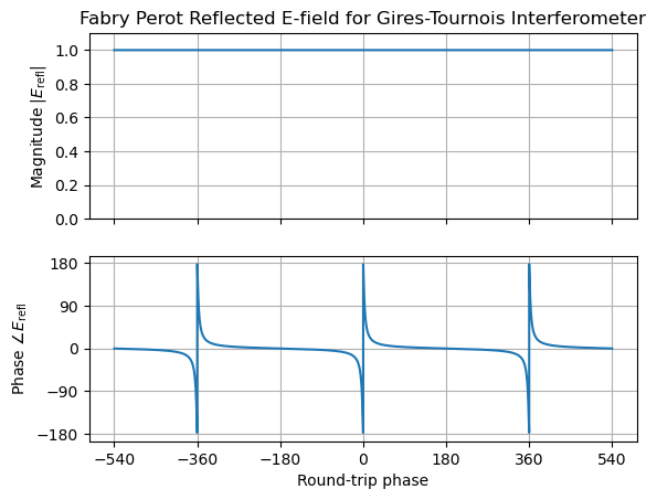
6 Reflection Phase Angle vs Frequency ¶ 6.1 Plots ¶ Make Bode plots of the reflection phase vs round-trip phase where ϕ \phi ϕ Hint: This is similar to our expressions θ ( ϕ ) \theta(\phi) θ ( ϕ ) θ \theta θ ϕ \phi ϕ
6.2 Reflection Phase Angle vs Frequency Solution ¶ The Fabry-Perot reflection field E r e f l E_\mathrm{refl} E refl
E r e f l = r 1 − r 2 e − i ϕ 1 − r 1 r 2 e − i ϕ \begin{align}
E_\mathrm{refl} = \dfrac{r_1 - r_2 e^{-i \phi}}{1 - r_1 r_2 e^{-i \phi}}
\end{align} E refl = 1 − r 1 r 2 e − i ϕ r 1 − r 2 e − i ϕ If R 2 = 100 % R_2 = 100\% R 2 = 100% r 2 = 1 r_2 = 1 r 2 = 1
E r e f l = r 1 − e − i ϕ 1 − r 1 e − i ϕ \begin{align}
E_\mathrm{refl} = \dfrac{r_1 - e^{-i \phi}}{1 - r_1 e^{-i \phi}}
\end{align} E refl = 1 − r 1 e − i ϕ r 1 − e − i ϕ Explicitly calculating the magnitude gives
∣ E r e f l ∣ = ∣ r 1 − e − i ϕ 1 − r 1 e − i ϕ ∣ = r 1 − e − i ϕ 1 − r 1 e − i ϕ r 1 − e i ϕ 1 − r 1 e i ϕ = r 1 2 + 1 − r 1 ( e i ϕ + e − i ϕ ) 1 + r 1 2 − r 1 ( e i ϕ + e − i ϕ ) = 1 \begin{align}
\left| E_\mathrm{refl} \right| &= \left| \dfrac{r_1 - e^{-i \phi}}{1 - r_1 e^{-i \phi}} \right|\\
&= \sqrt{ \dfrac{r_1 - e^{-i \phi}}{1 - r_1 e^{-i \phi}} \dfrac{r_1 - e^{i \phi}}{1 - r_1 e^{i \phi}} }\\
&= \sqrt{ \dfrac{r_1^2 + 1 - r_1 (e^{i \phi} + e^{-i \phi}) }{1 + r_1^2 - r_1 (e^{i \phi} + e^{-i \phi})} }\\
&= 1
\end{align} ∣ E refl ∣ = ∣ ∣ 1 − r 1 e − i ϕ r 1 − e − i ϕ ∣ ∣ = 1 − r 1 e − i ϕ r 1 − e − i ϕ 1 − r 1 e i ϕ r 1 − e i ϕ = 1 + r 1 2 − r 1 ( e i ϕ + e − i ϕ ) r 1 2 + 1 − r 1 ( e i ϕ + e − i ϕ ) = 1 But the phase is not trivial. Finding the real and imaginary parts of E r e f l E_\mathrm{refl} E refl
R e [ E r e f l ] = 1 2 ( E r e f l + E r e f l ∗ ) R e [ E r e f l ] = 2 r 1 − ( 1 + r 1 2 ) cos ( ϕ ) 1 + r 1 2 − 2 r 1 cos ( ϕ ) I m [ E r e f l ] = 1 2 i ( E r e f l − E r e f l ∗ ) I m [ E r e f l ] = ( r 1 2 − 1 ) sin ( ϕ ) 1 + r 1 2 − 2 r 1 cos ( ϕ ) \begin{align}
\mathrm{Re}[E_\mathrm{refl}] &= \dfrac{1}{2}( E_\mathrm{refl} + E_\mathrm{refl}^* )\\
\mathrm{Re}[E_\mathrm{refl}] &= \dfrac{2 r_1 - (1 + r_1^2)\cos(\phi)}{1 + r_1^2 - 2 r_1 \cos(\phi)}\\
~\\
\mathrm{Im}[E_\mathrm{refl}] &= \dfrac{1}{2i}( E_\mathrm{refl} - E_\mathrm{refl}^* )\\
\mathrm{Im}[E_\mathrm{refl}] &= \dfrac{ (r_1^2 - 1) \sin(\phi)}{1 + r_1^2 - 2 r_1 \cos(\phi)}\\
\end{align} Re [ E refl ] Re [ E refl ] Im [ E refl ] Im [ E refl ] = 2 1 ( E refl + E refl ∗ ) = 1 + r 1 2 − 2 r 1 cos ( ϕ ) 2 r 1 − ( 1 + r 1 2 ) cos ( ϕ ) = 2 i 1 ( E refl − E refl ∗ ) = 1 + r 1 2 − 2 r 1 cos ( ϕ ) ( r 1 2 − 1 ) sin ( ϕ ) So the argument of E r e f l E_\mathrm{refl} E refl
∠ E r e f l = 1 1 + r 1 2 − 2 r 1 cos ( ϕ ) arctan 2 [ ( r 1 2 − 1 ) sin ( ϕ ) , 2 r 1 − ( 1 + r 1 2 ) cos ( ϕ ) ] \begin{align}
\angle E_\mathrm{refl} = \dfrac{1}{1 + r_1^2 - 2 r_1 \cos(\phi)} \arctan2\left[(r_1^2 - 1) \sin(\phi) , 2 r_1 - (1 + r_1^2)\cos(\phi) \right]
\end{align} ∠ E refl = 1 + r 1 2 − 2 r 1 cos ( ϕ ) 1 arctan 2 [ ( r 1 2 − 1 ) sin ( ϕ ) , 2 r 1 − ( 1 + r 1 2 ) cos ( ϕ ) ] This result is plotted below.
def erefl(phi, trans1, trans2, ein=1):
    """Reflected electric field from a Fabry-Perot optical cavity Erefl
    Inputs:
    -------
    phi: float
        round-trip phase of the optical cavity
    trans1: float
        power transmission of the input mirror
    trans2: float
        power transmission of the end mirror
    ein: float
        input electric field, default is ein = 1 sqrt(W)

    Output:
    -------
    erefl: complex float
        complex reflection field from the Fabry Perot
    """
    r1 = np.sqrt(1 - trans1)
    r2 = np.sqrt(1 - trans2)
    erefl = (r1 - r2 * np.exp(-1j * phi))/(1 - r1 * r2 * np.exp(-1j * phi))
    return erefl
phis = np.linspace(-3*np.pi, 3*np.pi, 10000)
trans1 = 0.1 # input power transmission
trans2 = 0 # perfectly reflecting

erefls = erefl(phis, trans1, trans2)
import matplotlib.pyplot as plt
fig, (ax1, ax2) = plt.subplots(2, sharex=True)
ax1.plot(180/np.pi * phis, np.abs(erefls))
ax2.plot(180/np.pi * phis, np.angle(erefls, deg=True))
ax1.set_ylim(0, 1.1)
ax2.set_yticks([-180, -90, 0, 90, 180])
ax1.set_xticks(180*np.arange(-3,4))
ax1.grid()
ax2.grid()
ax1.set_title("Fabry Perot Reflected E-field for Gires-Tournois Interferometer")
ax1.set_ylabel(r"Magnitude $|E_\mathrm{refl}|$")
ax2.set_ylabel(r"Phase $\angle E_\mathrm{refl}$")
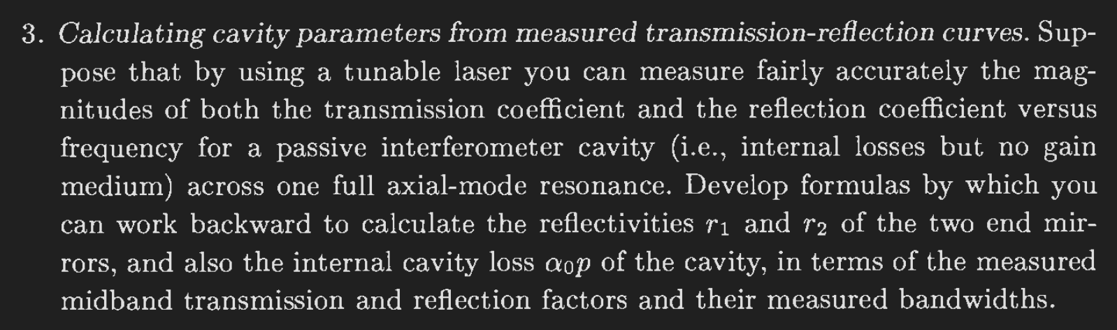
ax2.set_xlabel(r"Round-trip phase")7 Cavity Measurement and Modeling (Extra Credit) 