Michelson Interferometers, Modulations, and Transfer Functions - Homework 03

This is the third homework assignment for Lasers and Optomechanics at Syracuse University.
It is due Monday, March 02, 2026 by 5 pm

You will need to complete the questions in this jupyter notebook and submit it via gitlab

1Homodyne Michelson¶

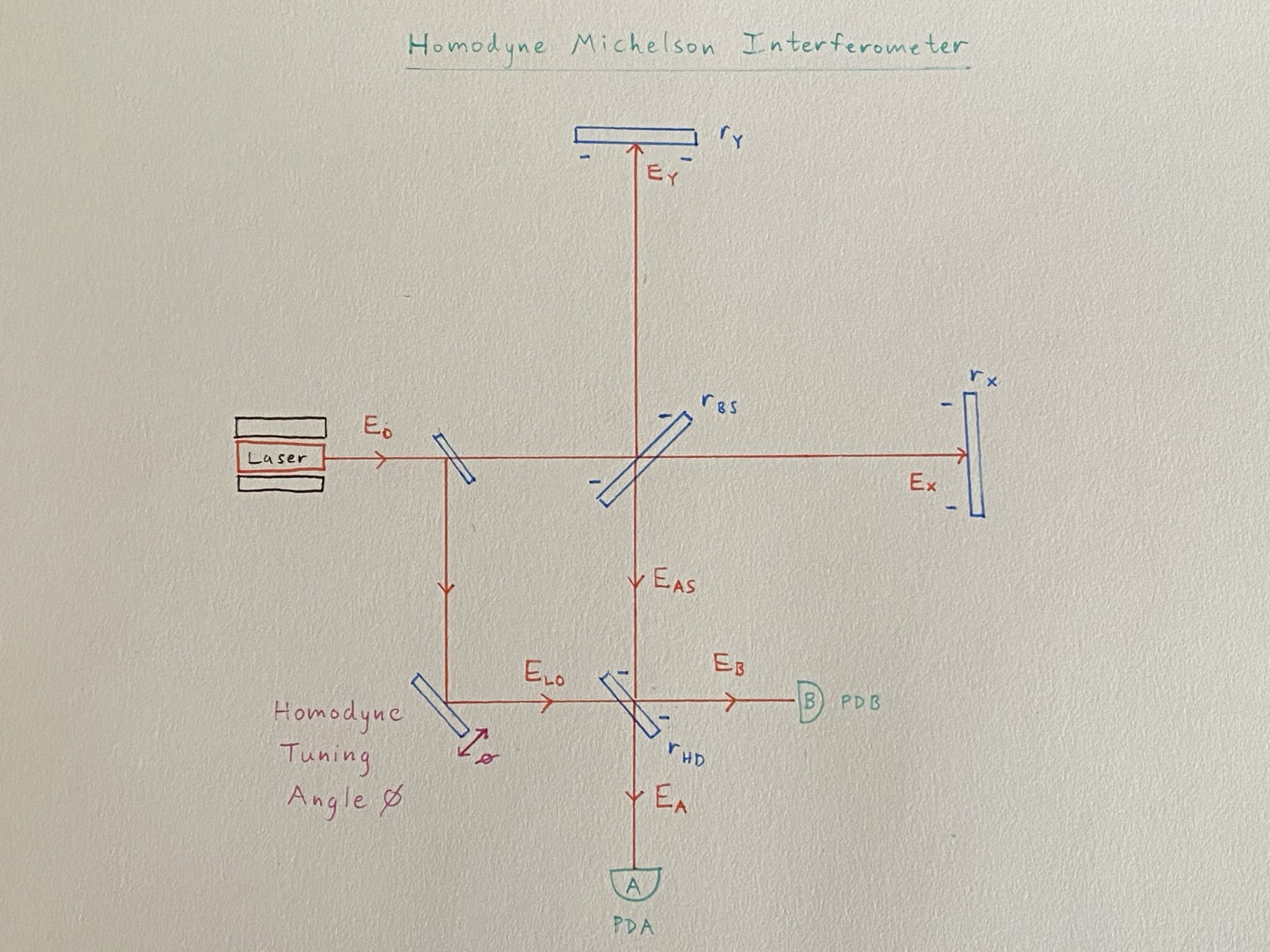
Homodyne Michelson Interferometer Diagram

1.1Adjacency Matrix¶

Set up an Adjacency Matrix $\boldsymbol{M}$ for the Homodyne Michelson.
You may choose any electric fields vector you want, but you have to include the explicitly labeled electric fields.
The homodyne angle $\phi_\mathrm{HD}$ can be considered as the total phase accrued by the local oscillator field $E_\mathrm{LO}$ in the pick-off path:

1.2Electric Field Transfer Functions¶

Invert your Adjacency Matrix minus the identity $(\boldsymbol{M} - \boldsymbol{I})^{-1}$ to calculate the transfer functions from each electric field to every other electric field.
Pick out the field transfer functions from the input to the photodetectors $\mathrm{PD}_A$ and $\mathrm{PD}_B$ $\dfrac{E_\mathrm{PDA}}{E_\mathrm{in}}$ and $\dfrac{E_\mathrm{PDB}}{E_\mathrm{in}}$.

1.3Substitutions¶

Apply the phase change of basis used in class $\phi_d = \dfrac{\phi_x - \phi_y}{2}$ and $\phi_c = \dfrac{\phi_x - \phi_y}{2}$ to your field transfer functions above.
You may also assume a perfect Michelson beamsplitter $r_\mathrm{BS} = t_\mathrm{BS} = \dfrac{1}{\sqrt{2}}$.

1.4Power Transfer Functions¶

Calculate the input to power transfer functions $\dfrac{P_\mathrm{PDA}}{P_\mathrm{in}}$ and $\dfrac{P_\mathrm{PDB}}{P_\mathrm{in}}$.

1.5Interpretation¶

How do $\dfrac{P_\mathrm{PDA}}{P_\mathrm{in}}$ and $\dfrac{P_\mathrm{PDB}}{P_\mathrm{in}}$ depend on the homodyne angle $\phi_\mathrm{HD}$, and the common and differential Michelson phase $\phi_d$ and $\phi_c$?
Can we manipulate the homodyne angle $\phi_\mathrm{HD}$ to detect the differential phase $\phi_d$?
Can you think of any problems you might run into if you tried to actually set up a homodyned Michelson?

2Homodyne Michelson Solution¶

2.1Part A: Adjacency Matrix¶

First, create the electric field vector $\vec{E}$, with elements below

Optical elements:

• $M_1$: Input beamsplitter (splits signal/LO), coefficients $(r_{m1},\, t_{m1})$

• $M_2$: Homodyne steering mirror (imparts LO phase $\phi_\mathrm{hd}$), coefficient $r_{m2}$

• $M_3$: Homodyne beamsplitter (combines $E_\mathrm{as}$ and $E_\mathrm{lo}$), coefficients $(r_\mathrm{hd},\, t_\mathrm{hd})$

The $10\times10$ adjacency matrix, with rows/columns ordered $E_1,\ldots,E_{10}$, is:

Reading off this matrix, for example $E_{10} = -r_\mathrm{hd} E_7 + t_\mathrm{hd} E_8$.
This matches with what we might read off the diagram, with $E_{10} = E_B$, $E_7 = E_{as}$, $E_8 = E_{lo}$, yielding

Inverting this matrix minus the identity gives us our transfer functions:

2.2Part B: Electric Field Transfer Functions¶

From our matrix inversion, we can pick off the last two rows and first column elements $G_{9,1}$ and $G_{10,1}$

2.3Part C: Substitutions¶

Physically motivated simplifications:

1. Phase basis change: $\phi_x = \phi_c + \phi_d$, $\;\phi_y = \phi_c - \phi_d$

2. Ideal 50:50 Michelson BS: $t_\mathrm{bs} = r_\mathrm{bs} = 1/\sqrt{2}$

3. Perfect end mirrors: $r_x = r_y = 1$,

4. Perfect steering mirror: $r_{m2} = 1$

5. Ideal 50:50 homodyne BS: $t_\mathrm{hd} = r_\mathrm{hd} = 1/\sqrt{2}$

6. Ideal 50:50 input BS: $t_{m1} = r_{m1} = 1/\sqrt{2}$

2.4Part D: Power Transfer Functions¶

(Assume that $E_\mathrm{in} = 1~\sqrt{\mathrm{W}}$ and $P_\mathrm{in} = 1~\mathrm{W}$)

Derivation for $P_A$:

The normalised powers $P_A = \left|E_A\right|^2$, $P_B = \left|E_B\right|^2$ are :

Analyzing the above, what is actually most useful as an error signal is the power sum $P_\mathrm{sum} = P_A + P_B$ and difference $P_\mathrm{diff} = P_A - P_B$:

Setting $\phi_\mathrm{hd} = 2\phi_c - \pi/2$ maximises sensitivity to $\phi_d$:

2.5Plots¶

Plot 1: Power vs Differential Phase $\phi_d$¶

Optimal homodyne angle $\phi_\mathrm{hd} = 2\phi_c - \pi/2$, with $\phi_c = 0$.

$P_A - P_B = \sin(2\phi_d)$ crosses zero at $\phi_d = 0$, providing a linear error signal for dark-fringe locking.

Plot 2: Power vs Common Phase $\phi_c$¶

$\phi_d = \pi/4$ (bright Michelson), $\phi_\mathrm{hd} = 0$.

The common phase $\phi_c$ redistributes power between detectors A and B, but leaves the sum $P_A+P_B$ unchanged.

Plot 3: Power vs Homodyne Angle $\phi_\mathrm{hd}$¶

$\phi_d = \pi/4$ (bright Michelson), $\phi_c = 0$.

Sweeping $\phi_\mathrm{hd}$ rotates the interference between $E_\mathrm{as}$ and $E_\mathrm{lo}$, shifting signal between detectors while keeping the sum constant.

Note: This sweep only works on a bright fringe -- if the Michelson is dark ($E_\mathrm{as}=0$), the LO has nothing to beat against. This motivates the coherent locking field (CLF): an RF-modulated sideband co-propagating with squeezed light that provides a homodyne angle reference even on the dark fringe.

2.6Extra Credit: Optimal Input Beamsplitter Ratio¶

Relaxing the 50:50 assumption on $M_1$ (keep $r_{m1}$, $t_{m1}$ free, $r_{m1}^2 + t_{m1}^2 = 1$), gives new expressions for $E_A$ and $E_B$:

Turning the crank:

At the optimal homodyne angle $\phi_\mathrm{hd} = 2\phi_c - \pi/2$, the differential signal becomes:

Maximising over $T_{m1} \equiv t_{m1}^2$ (with $r_{m1} = \sqrt{1-T_{m1}}$):

A 50:50 input beamsplitter gives the maximum sensitivity to differential phase.

3Asymmetric Michelson¶

Suppose you have a Michelson interferometer with the X-arm much longer than the Y-arm:

In this problem, we will calculate the full frequency response transfer functions of the Michelson

I recommend using an algebra helper like Mathematica or sympy for this problem. You may convert your answers to LaTeX using TeXform in Mathematica or some such similar function for sympy.

3.1Field tranfer functions¶

Derive the electric field transfer functions for the following:

where $E_\mathrm{in}$ is the input electric field $E_0 e^{i \omega_0 t}$,
$E_\mathrm{x}$ is the field reflected from the X-arm mirror,
$E_\mathrm{y}$ is the field reflected from the Y-arm mirror,
and $E_\mathrm{as}$ is the field at the antisymmetric (or transmission) port.

Use $r_\mathrm{bs}, t_\mathrm{bs}$ for the beamsplitter reflection and transmission,
$r_\mathrm{x}, r_\mathrm{y}$ for the X and Y mirror reflections, and
$\phi_x, \phi_y$ for the single-pass phase accrued by the field as it propagates in the X-arm or Y-arm.

3.2End Mirror Modulation¶

Now, suppose we apply some common modulation to both end mirrors:

Write what the new arm reflected transfer functions are for:

Hint: Remember that you should end up with three distinct fields at $\omega_0$ and $\omega_0 \pm \omega$

3.3Propagate to the antisymmetric port¶

Propagate your new transfer functions to the antisymmetric port, and compute a new $\dfrac{E_\mathrm{as}}{E_\mathrm{in}}$.

Be careful here.
Consider carefully what $k = \omega/c$ is for each of your electric fields as they propagate back to the beamsplitter, accruing some phase $\phi = -k L$.
Should each field accrue the same phase?

3.4Calculate the power response¶

Calculate the power response to the common motion $\dfrac{P_\mathrm{as}}{P_\mathrm{in}}$.

This is a lot of algebra, I recommend Mathematica or sympy to help you make sure you get things right here.
You may find it useful to express your arm phases in the common and differential bases again, since you have already incorporated the time-dependent term $\Gamma \cos(\omega t)$ as two additional sideband terms:

You may assume an ideal beamsplitter

and balanced arms

and small modulation from the end mirrors

Answer:

3.5Demodulate the power term¶

Calculate

by integrating $P_\mathrm{as}$ over one cycle of $\omega t$ while multiplying by $1, \cos(\omega t)$ and $\sin(\omega t)$, respectively.

Does your answer for $P_\mathrm{as}^\mathrm{DC}$ seem familiar?

3.6Caluculate the Frequency Response to CARM motion in an Asymmetric Michelson¶

Calculate the frequency response

to CARM motion $\Gamma$.

Plot the magnitude and phase for $\dfrac{P_\mathrm{as}}{\Gamma}(\omega)$.

Assume

4Asymmetric Michelson Solution¶

4.1Part A: Electric Field Transfer Functions¶

The field transfer functions for the Michelson are

where $E_\mathrm{in} = E_0 e^{i \omega_0 t}$ is the input electric field,\ and $\phi_x = k L_x$ and $\phi_y = k L_y$ are the single pass phase accrued from traversing the arms.
For us, $L_x > L_y$, so the raw amount of phase accrued in each arm is very different,but our basis breakdown still works.
We can still write down $\phi_c = \phi_x + \phi_y$ and $\phi_d = \phi_x - \phi_y$, and assuming $r_y = r_x$, rewrite $E_{as}$ in the new basis:

For the rest of this problem, $\phi_x$ and $\phi_y$ will be broken down into a DC term $\phi_{x0}, \phi_{y0}$, and an AC, or modulating term $\phi_x(t),\phi_y(t)$:

4.2Part B: Modulation applied to the end mirrors¶

From class, we saw that mirror motion is equivalent to phase modulation.
Here we apply a common phase modulation of $\phi_c(t) = 2 \Gamma \cos(\omega t)$,
so $\phi_x(t) = \phi_y(t) = \Gamma \cos(\omega t)$,
where $\Gamma$ is the modulation depth in radians,
$\omega$ is the modulation frequency in radians/second,
and $t$ is time.

For the beam immediately reflected off the X-arm, we get three frequencies of light coming back, at $\omega_0$, and $\omega_0 \pm \omega$:

Notice that all the beams have experienced the same phase delay $\phi_{x0} = k L_x = \omega_0 L_x / c$ at the end mirror,
represented by this common coefficient $e^{-i \phi_{x0}}$,
because during the time the beam propogated to the end mirror, there was only one frequency of light $\omega_0$.

Similarly for the Y-arm:

In the last step for both, I distributed the $e^{i \omega_0 t}$ term to each of the three fields to emphasize their actual propagation frequency.

4.3Part C: The Dark Port Field $E_{as}$¶

Now, let’s propogate the beams back to the beamsplitter.
We need to calculate

where $E_{x2}$ and $E_{y2}$ are the beams incident on the backside of the beamsplitter.

X-arm¶

First we’ll focus on calculating $E_{x2}$ from our $E_x$ above. The key difference here is we have our three beams propogating back to the beamsplitter across the same space, but now will experience different phase accretion.

Recall that the propagation coefficient is $e^{-i k L_x}$. In this case, we have three different $k$, because $k = \Omega / c$, and we have $\Omega = {\omega_0, \omega_0 + \omega, \omega_0 - \omega}$.
(Here I used $\Omega$ to represent a generalized frequency, because $\omega$ is already taken for our modulation frequency).

So, our carrier, upper sideband, and lower sideband will experience three different phases going back to the beamsplitter from the X-arm end mirror:

so the carrier accrues the exact same phase going back to the beamsplitter, but the sidebands accrue more or less phase.

I like to rewrite the sideband phases accrued in terms of the carrier DC phase $\phi_{x0}$ and $\omega$:

Reproducing our expression for $E_{x}$:

Now we apply our additional propagation delays to each beam to get $E_{x2} = e^{-i k L} E_{x}$: