Transmission Dither Locking, Pound-Drever-Hall Michelson, and Fabry-Perot Michelson - Homework 04

This is the fourth homework assignment for Lasers and Optomechanics at Syracuse University.
It is due Monday, April 6th, 2026 by 5 pm

You will need to complete the questions in this jupyter notebook and submit it via gitlab

1Transmitted Field Dither Locking¶

In class, we investigated dither locking using the reflected field $E_\mathrm{refl}$ from a Fabry-Perot cavity.

In this problem, investigate whether it is possible to use $E_\mathrm{trans}$ to hold lock.

1.1Plot of Fabry-Perot $E_\mathrm{trans}$ versus $E_\mathrm{trans}$¶

Plot both $E_\mathrm{refl}$ and $E_\mathrm{trans}$ over a span of $\phi \in \left[ -\dfrac{\pi}{2},\dfrac{3\pi}{2} \right]$

Do you notice anything different about the resonance points?

1.2Total $E_\mathrm{trans}$ with end-mirror moduation¶

If we apply an end-mirror modulation $\Delta x \cos(\omega t)$ to our Fabry-Perot cavity, what is the total $E_\mathrm{trans}(t)$ field?

1.3Calculate the total transmitted power $P_\mathrm{trans}(t)$¶

Calculate $P_\mathrm{trans}(t) = |E_\mathrm{trans}(t)|^2$

You may set $\Delta x^2 = 0$ for simplicity in the calculations.
You should end up with only DC and 1$\omega$ terms.

You may leave this power term in a general form if you wish, but you must be clear what each of the contributing fields are.

1.4Calculate the transmitted power demodulated at $\omega$¶

Calculate the demodulated term $P_\mathrm{trans}(\omega) = P^I_\mathrm{trans}(\omega) + i P^Q_\mathrm{trans}(\omega)$. This should be directly proportional to $\Delta x$.

1.5Plot the length to transmitted power function phase sweep¶

Plot the real and imaginary parts of $\dfrac{P_\mathrm{trans}(\omega)}{\Delta x}$ over $\phi \in \left[ -\dfrac{\pi}{2},\dfrac{3\pi}{2} \right]$

Choosing some low to moderate finesse cavity parameters, plot your derived function $\dfrac{P_\mathrm{trans}}{\Delta x}(\omega)$ as a function of carrier phase $\phi$.

Let the cavity parameters be

1.6Plot the length to transmitted power transfer function¶

Plot your transfer function magnitude and phase $\dfrac{P_\mathrm{trans}}{\Delta x}(\omega)$ as a function of frequency $f = \omega / (2\pi)$.

Use the same cavity parameters as above, but allow $f \in [3 \times 10^3, 3 \times 10^8]~\mathrm{Hz}$, while setting $\phi = 1^{\circ}$.

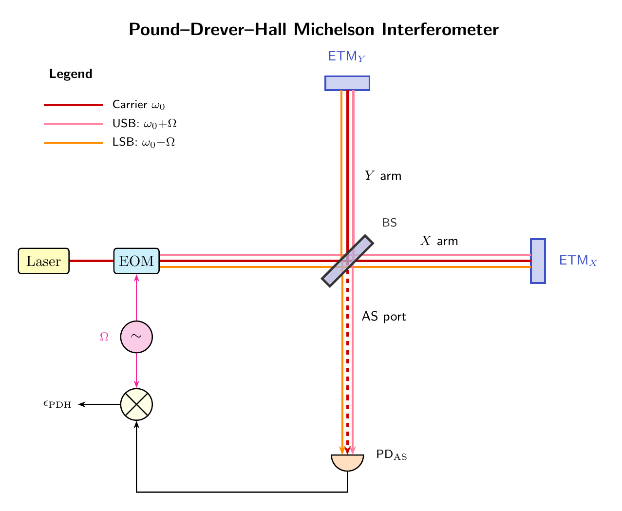
2Pound-Drever-Hall Michelson¶

In-class we went over the Pound-Drever-Hall (PDH) Fabry-Perot interferometer.

Now we’ll try to apply the same technique lock a Michelson interferometer to it’s carrier dark fringe.

Below is a diagram of a Michelson with carrier at $\omega_0$, and two RF phase sidebands created by an electro-optic modulator (EOM) oscillating at $\Omega$ to create two frequencies $\omega_0 \pm \Omega$.
Our goal is to calculate the PDH error signal $\epsilon_\mathrm{PDH}$ as a function of the carrier phase offset $\phi_d$ and RF sideband frequency $\Omega$.

2.1Calculate the total dark field $E_{as}(t)$.¶

Calculate the full field expression $E_{as}(t)$ at the dark port of the interferometer.

There should be three contributions, one from carrier and two from the RF phase sidebands injected alongside the carrier.

Let the modulation depth of the RF sideband be $\Gamma$.
Let the carrier differential phase be $\phi_d = \omega_0 (L_x - L_y) / c$,
and the RF phase differential phase be $\varphi_d = \Omega (L_x - L_y) / c$.\

What happens to our phases and $E_{as}(t)$ if $L_x = L_y$ exactly?

Hint: The RF sidebands will experience a phase shift of $\phi_d \pm \varphi_d$ as it transmitted through the interferometer

2.2Calculate the total dark power $P_{as}(t)$.¶

Calculate $P_{as}(t) = |E_{as}(t)|^2$.

Assume that the second order modulation terms $\Gamma^2 = 0$, for simplicity.

2.3Calculate the dark power demodulated at $\Omega$¶

Calculate and plot the phase sweep of $\dfrac{P_{as}}{\Gamma}(\phi_d, \varphi_d)$ for $\phi_d \in [-5\pi, 5\pi]$. for some assumed cavity parameters:

What do you notice about this signal $\dfrac{P_{as}}{\Gamma}(\phi_d, \varphi_d)$ as we increase the offset $\phi_d$?

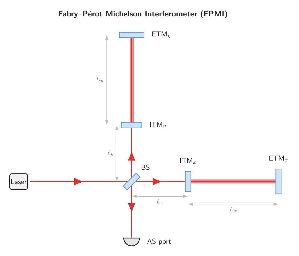
3Fabry-Perot Michelson Interferometer (FPMI)¶

We investigated compound interferometers in class when we studied the coupled-cavity.
Here we combine our Michelson interferometer with Fabry-Perot interferometers forming the arms, forming the Fabry-Perot Michelson Interferometer (FPMI) in a configuration similar to LIGO.

3.1Adjacency Matrix¶

Form an adjacency matrix for the FPMI interferometer.

I recommend using $\phi_x = k \ell_x$ and $\phi_y = k \ell_y$ for the short Michelson arms,
and $\Phi_x = k L_x$ and $\Phi_y = k L_y$ for the Fabry-Perot arm lengths.

3.2Antisymmetric Port Field Derivations¶

Find the $\dfrac{E_\mathrm{as}}{E_\mathrm{in}}$ transfer function by inverting the adjacency matrix.

You may also derive the FPMI response by using the compound interferometer technique, by letting the common Michelson X-arm reflection $r_x \rightarrow r_\mathrm{FP}(\Phi_x) = \dfrac{E_\mathrm{refl}}{E_\mathrm{in}}$.
Does this derivation agree with your result from the adjacency matrix?

3.3Simplifications to $E_\mathrm{as}$¶

At this point, you may simplify $E_\mathrm{as}$ and change the basis using

The above assumes the short Michelson is always perfectly tuned, and the beamsplitter is ideal, and the Fabry-Perot arms are ideally balanced.

3.4Interpretation¶

Plot the real and imaginary parts of $\dfrac{E_\mathrm{as}}{E_\mathrm{in}}$ as a function of $\Phi_d$.

Compare to the normal Michelson solution for the AS port.
Do the Fabry-Perot arms enhance our sensitivity to differential displacement $\Phi_d$?

You may substitute in a moderate finesse Fabry-Perot cavity values