Photons and Lasers

1Readings:¶

Reading 1: Chapter 1 of Lasers by Siegman

(Fun) All is not right with Classical Mechanics:
Link 2: Chapter 3 of Shankar

(Optional) Quantum Optics intro:
Link 2: Chapter 2.1 of Gerry and Knight Introductory Quantum Optics

(Optional) Review of Griffith’s QM:
Link 3: Chapter 2.3 of Griffith’s QM

2Photons: A Qualitative Overview¶

Light is famously made of photons, which act as the force carriers for the electromagnetic field in the standard model.
A photon of light carries energy $E_\omega = \hbar \omega$, where $\hbar$ is the reduced Planck’s constant and $\omega$ is the angular frequency of the light wave.

2.1Harmonic Oscillator Review¶

From Griffith’s Quantum Mechanics Chapter 2.3,
for a harmonic oscillator with potential $V(x) = \dfrac{1}{2} m \omega^2 x^2$,
the energy levels are separated by $E = \hbar \omega$.

As it turns out, electric and magnetic fields can be quantized.
As we’ve seen in the previous lecture, Maxwell’s equations for electric and magnetic fields yield harmonic oscillator solutions,
with eigenstates $|n \rangle$ with energy $E_n = \left(n + \dfrac{1}{2} \right) \hbar \omega$.

Crucially, the ground state $|0 \rangle$ is non-zero energy, and while the mean energy is zero, the variance in the ground state is non-zero, leading to measurable fluctuations in the field.

See Link 3: Chapter 2.1 of Gerry and Knight Introductory Quantum Optics for an overview.

This is not a quantum optics class, so I will not emphasize the discrete nature of light,
but we will need to remember the quantum nature of light when calculating shot noise or talking about squeezing later on.

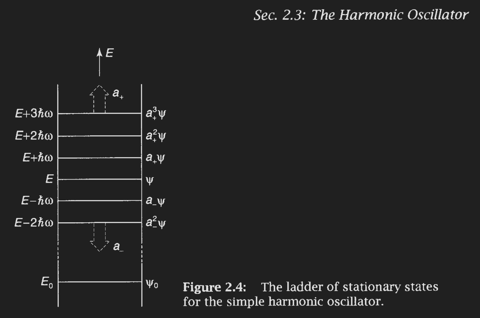
Energy ladder for a harmonic oscillator from Griffith’s QM.

2.2Hydrogen Atom Energy Levels¶

Quanta of light energy can be emitted via transitions in energy levels inside atoms, molecules, etc. The simplest real-world example is derived in introductory quantum mechanics books: the hydrogen atom.

In Chapter 4 of Griffith’s QM, spherical coordinates and the Coulomb potential $V(r) = - \dfrac{e^2}{4 \pi \epsilon_0}\dfrac{1}{r}$ are used to directly derive the quantum states and energy levels of the hydrogen atom. The differences in the energy levels are then observed as the photons emitted when the hydrogen atom is excited.

All quantum system (atoms, molecules) have distinct energy levels, and therefore distinct energy level transitions.
These transitions can be exploited to produce lots of light of the same kind.
This is the fundamentals of lasers.

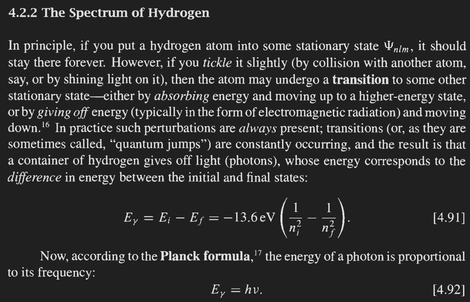
Energy level equations of the hydrogen atom, taken from Griffith’s QM Chapter 4

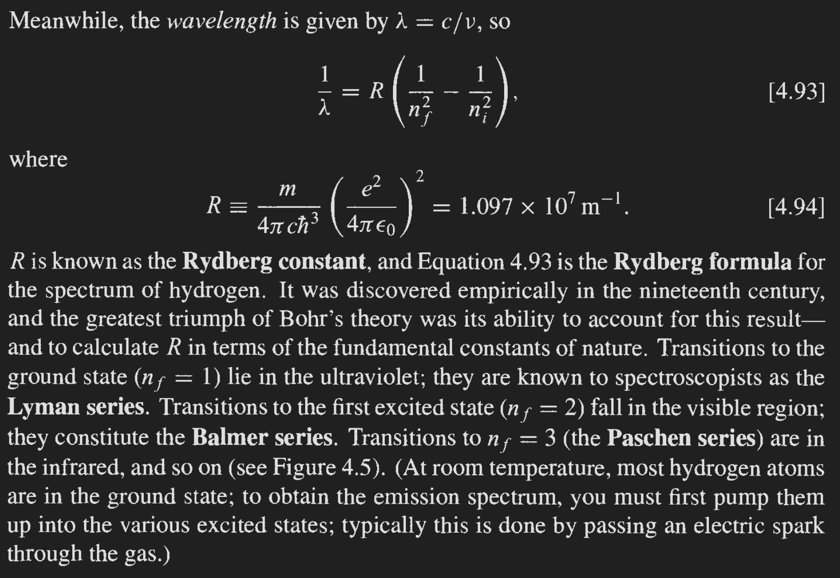
Energy level transitions descriptions, taken from Griffith’s QM Chapter 4

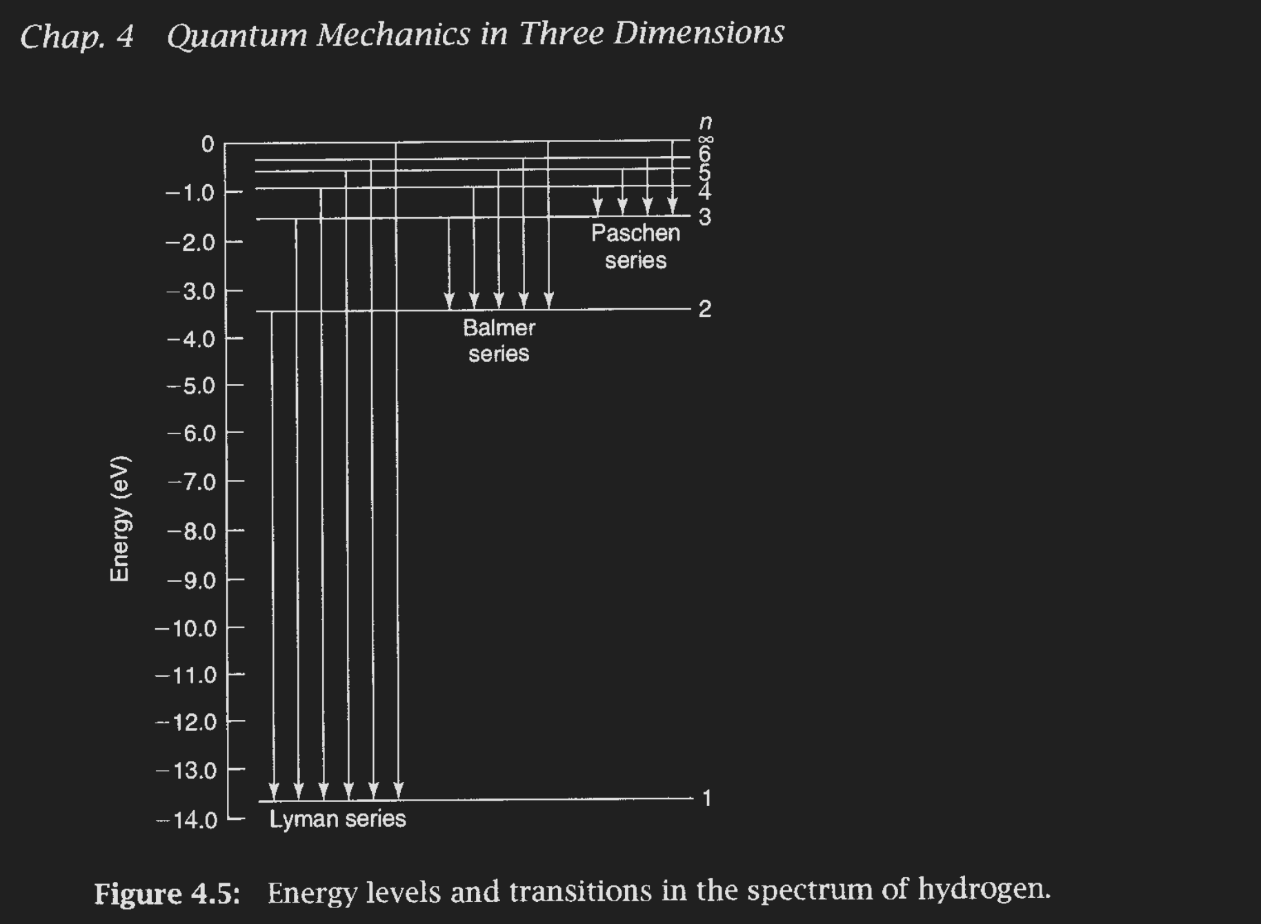
Energy level transitions of the hydrogen atom, taken from Griffith’s QM Chapter 4

2.3Quantum Mechanics Review¶

1. Maxwell’s equations allow for any amount of energy in light waves.
   Planck’s Law of quantum mechanics limits us to discrete light particles called photons, each with energy $E = \hbar \omega$, where $\hbar$ is a very small number and $\omega$ is the light frequency.

2. We can increase the total energy of light by stacking many photons: $E_\mathrm{total} = n \hbar \omega$, where $n$ is the number of photons available.

3. Quantum effects typically start becoming important when $n = 0$ or $n = 1$.
   Otherwise light can be considered to behave semiclassically.
   It is in the semiclassical limit we will mostly operate.

4. The hydrogen atom energy level transitions define what energies of light hydrogen can absorb and emit.
   The hydrogen atom cannot interact with other energies of light, those simply pass directly through hydrogen.

5. Other atoms have different energy levels, and therefore different transitions and different frequencies of light they can interact with.

3Lasers¶

Here we will review some important aspects of lasers as presented in Chapter 1 of Lasers by Siegman.

A laser is a device that generates or amplifies coherent light at the same frequency. These laser frequencies of emission are sometimes called lines. The term line referring to a spectral breakdown of the laser’s emission, where a high emission creates a strong output at a specific frequency, creating a line on the graph.

Any laser must be comprised of three elements:

1. A gain medium consisting of an appropriate collection of atoms, molecules, ions, or in some instances a semiconducting crystal;

2. A pumping process to excite these atoms (molecules, etc.) into higher quantum-mechanical energy levels;

3. Optical feedback elements that allow a beam of radiation to either pass once through the laser medium (as in a laser amplifier) or bounce back and forth repeatedly through the laser medium (as in a laser oscillator).

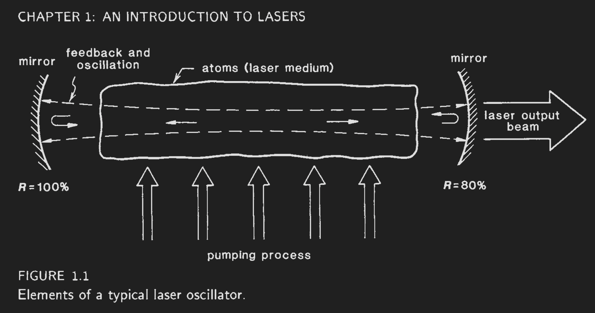
A laser oscillator system comprised of two mirrors around a lasing medium, from Chapter 1 of Lasers by Siegman.

3.1Laser Pumping and Population Inversion¶

For a laser to be effective, the source of energy to power the laser must be primed by the pumping process to allow for the desired photons to be created.

Population inversion refers to the elevation of the gain medium into an semi-stable excited state, where most of it’s atoms are in an excited state compared to the atoms in the ground state. The semi-stable excited state means that the gain medium doesn’t immediately return to it’s ground state via spontaneous emission: it holds onto it’s energy until encouraged to release it via stimulated emission.

The number of atoms in the excited state $N_2$ must be greater than the number of atoms in the ground state $N_1$ for the population to be inverted:

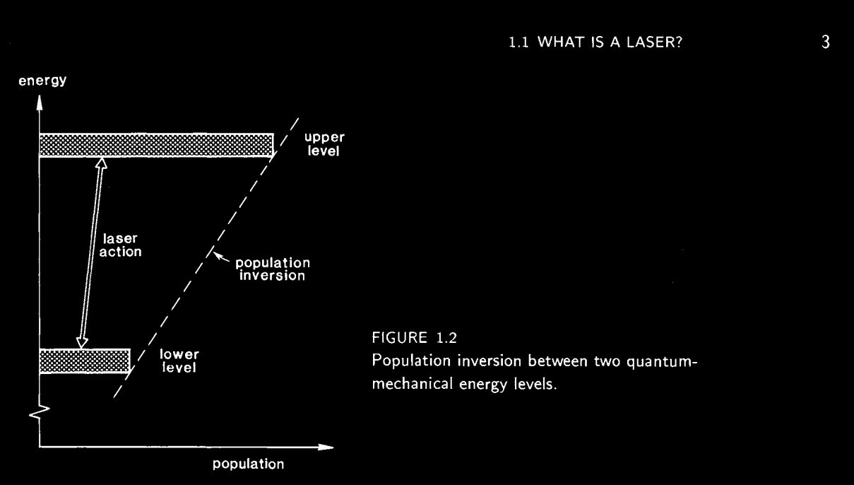
From Chapter 1 of Siegman’s Lasers

3.2Types of Lasers¶

A laser medium, or gain medium is usually defined by the active material inside the medium, i.e. the atoms or molecules defining the energy levels. This can take on many forms:

1. In a gas laser, the gas defines the laser emission. A common example is the Helium-Neon (HeNe) laser. The helium gas gets excited, bumps into neon gas, which then emits a red line at 633 nm.

2. In a diode laser, or semiconductor laser, the bandgap energy between the electron conduction bands or bound states of the semiconductor define the lasing possibilities. These are typically electrically pumped, and are newer and capable of delivering large amounts of laser power.

3. In a solid-state lasers, a glass (ruby) or doped-crystal (ytterbium) acts as the gain medium. Solid-state can be either optically or electrically pumped.

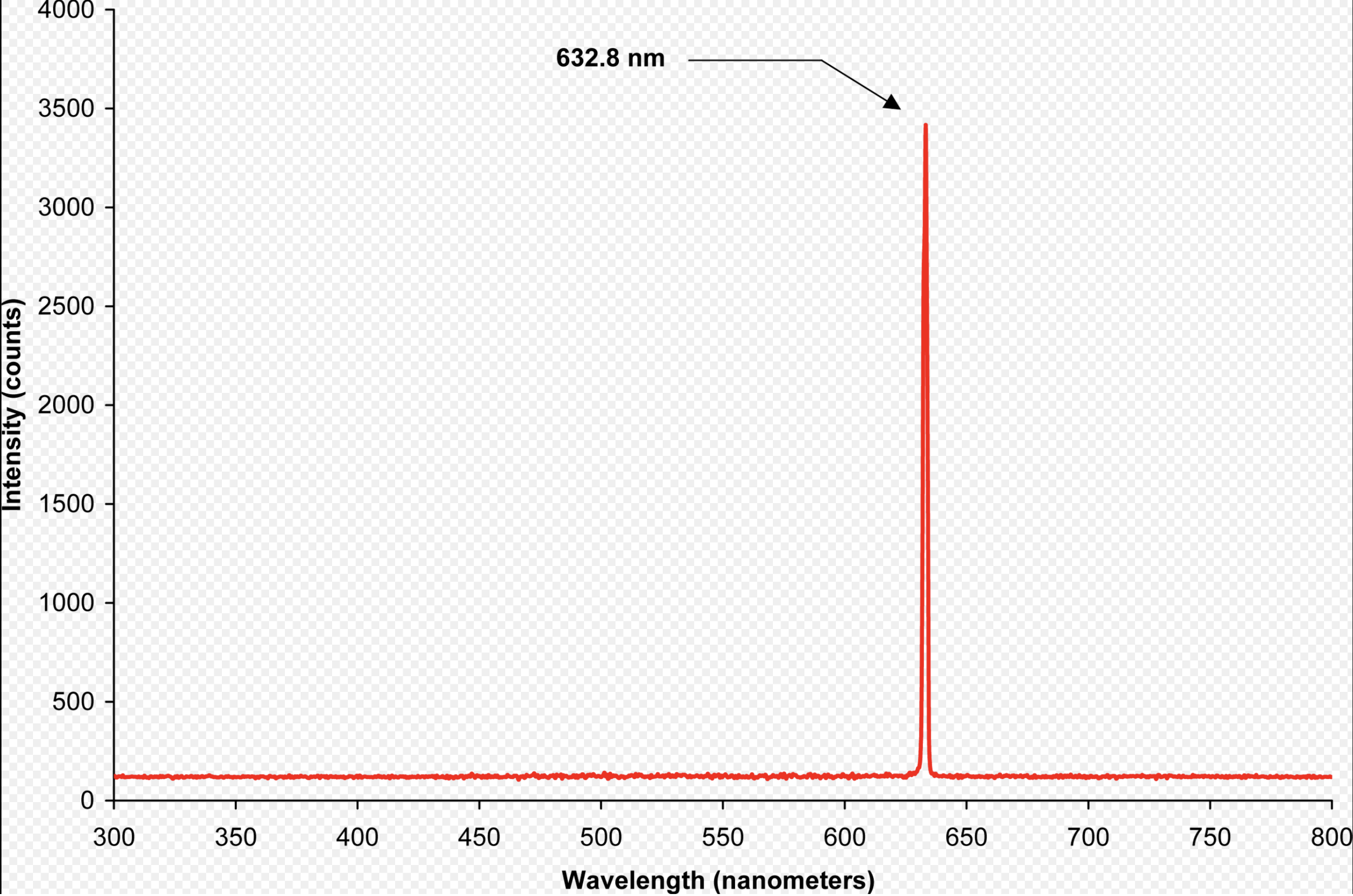
Helium-Neon laser line centered at 633 nm, a common and useful bright red visible laser line.

3.3Spontaneous emission¶

Spontaneous emission is the random emission of light from an excited atom or material.
Spontaneous emission is the sort of light given off by blackbody radiation, which comes from the vibrational motion of charged particles creating photons to give off energy.

Any material pumped with energy wants to give their excess energy off any way it can.
Transitions of atoms down to lower energy levels is unavoidable for a excited gain medium. All possible transitions down the energy ladder are taken.

The only transitions of interest will usually be the main laser transitions, that is, the transition from the main upper to the main lower state of our laser’s gain medium. These will emit photons close to, but not exactly the same as, our laser, creating fluctuations in the phase and amplitude of our laser.

3.4Absorption¶

The energy level diagrams of an atom are a two-way street. Photons of the correct energy incident upon an atom may be absorbed to kick an electron up from a lower energy level to a higher one. This process of photon annihilation is called absorption.

Spontaneous emission and absorption are the two directions an atom can travel on the energy ladder without the influence of other photons.

We can model the absorption $\alpha(\omega)$ of an electric field $E(z) = E_0 e^{-\alpha(\omega) z}$ over distance $z$ through some medium,
where

where $\lambda$ is the laser wavelength,
$\gamma_\mathrm{rad}$ is the radiative decay rate,
$\Delta \omega_a$ is the atomic linewidth,
and $\omega_{21}$ is the center frequency of the atomic line.\

The key here is the atomic population difference $N_1 - N_2$ in the numerator.
In a normal room-temperature situation with no pumping, $N_1 > N_2$, so $\alpha(\omega)$ will be positive.
However, if the population is inverted such that $N_1 < N_2$,
then this absorption coefficient becomes negative and becomes an emission coefficient.

This can lead to laser amplification through stimulated emission.

3.5Stimulated Emission¶

The core mechanism behind lasers is stimulated emission. Stimulated emission is the process of using one photon to generate an exact copy of itself from an excited (or pumped) atom. The copy photon has the same

1. frequency $\omega_0$,

2. polarization $\vec{e}$,

3. momentum $\vec{p} = \hbar \vec{k}$, and

4. phase $\phi$

as the original photon.

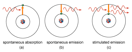
Stimulated versus spontaneous emission

Because all of the copied photons have the exact same properties, we are essentially building up enormous photon numbers $n$ all exactly in phase.
If the gain medium population inversion is set up, then the gain medium’s atoms cascade down to the lower energy level in concert, creating an enormous amount of photons with the same properties. If an oscillator and continuous pumping is set up, then the cascade can be sustained.
This can produces our steady power lasing field, called continous wave.

Pulsed lasers are brief, extremely powerful bursts of laser light. Laser pulses come from pumping up a massive excited population, then cascading the population down all at once, usually through a small seed pulse. Ultrafast laser pulses are extremely useful, used in laser cutting and inertial fusion confinement experiments like the National Ignition Facility.

Equation (2) for absorption also describes stimulated emission when the population inversion $N_2 > N_1$ occurs.
Equation (2) defines an atomic resonance of the laser’s gain media,
for which an incident beam of light will be amplified or absorbed.
Typically, the laser oscillator linewidth will be smaller than the atomic resonance

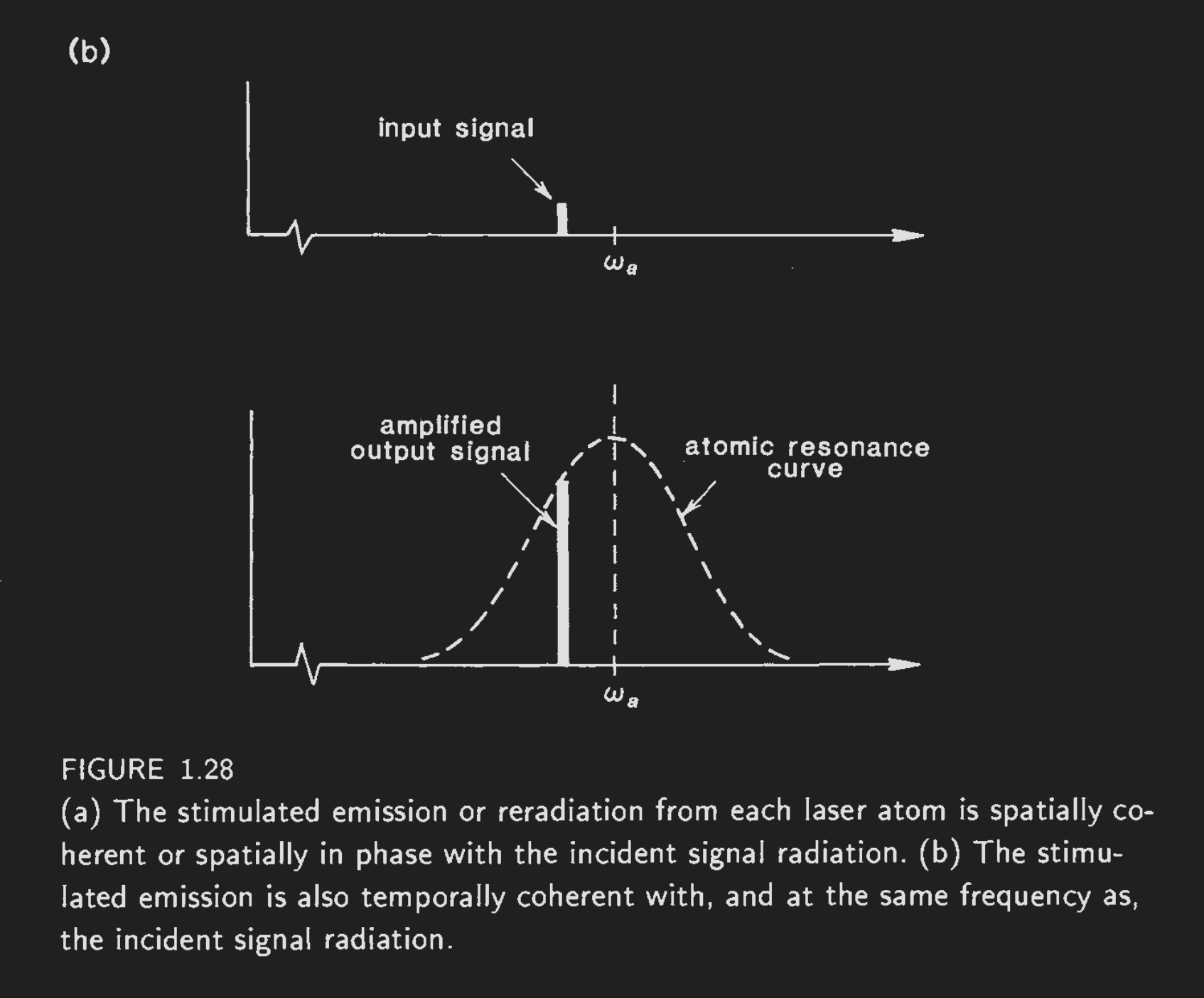Atomic resonance interacting with an incident beam of light, producing an amplifed beam.

In reality, not everything about the stimulated copies can be perfect.
Imperfections in the gain medium create small differences in the laser light over time and space. This leads to important effects that we will discuss later, including

1. Intensity (or amplitude) noise

2. Frequency (or phase) noise

3. Beam jitter

4. Non-gaussian laser beam profile

Three-level Systems¶

A three-level system is very convenient method of generating a semi-stable population inversion for your laser. In general, multiple levels are possible and commonly among laser media.

The energy ladder of an atom gives us a two-way street we can travel. In normal circumstances, any photon that is emitted by an atom can be absorbed by the next atom over. This is why population inverstion $N_2 > N_1$ is imperative to setting up a laser: the gain medium must prefer downward transitions to upward ones.

A two-level system can never give us an appropriate sytem for lasing. In a two-level system, there is no opportunity to achieve population inversion via pumping: any pump would be just as likely to excite an atom as it was to relax it.

Typically, a three-level system is electrically or optically pumped up to an upper state.
Then, a low-energy non-radiative energy decay to a slightly lower metastable energy level occurs. Finally, the output laser is emitted via stimulated emission.

The energy difference between the pump and the output laser is called the quantum defect. This energy is usually absorbed by the medium itself as heat.

Four-level or multi-level systems are also extremely common, one is shown below:

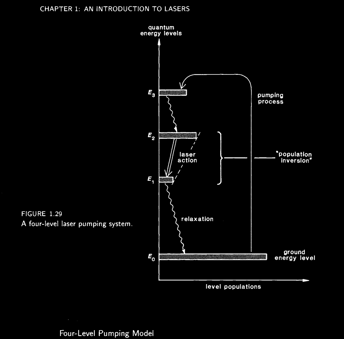
Four-level energy system with pumping to upper energy level, and non-radiative and radiative decay back down to the ground state (from Siegman Lasers Chapter 1.5)

Atomic Rate Equations¶

Suppose we have a number of atoms in the ground state $N_1(t)$ with energy $E_1$, and a number of atoms in the excited state $N_2(t)$ with energy $E_2$.

Both $N_1(t)$ and $N_2(t)$ are functions of time, and depend on the pumping power, spontaneous decay rates, and photons of energy $E_2 - E_1$ in the system.

Spontaneous Emission Rate¶

The spontanous emission depends only on the number of atoms in the excited state $N_2$, and decays like

where $t$ is time and $\gamma_{21}$ is the spontaneous decay rate.

Since the total number of atoms is conserved over time, and $N = N_1 + N_2$, we can write the above as

Absorption Rate¶

Suppose now we have $n(t)$ photons per unit volume inside of the gain medium. Suppose further that these are signal photons, i.e. ones close enough in energy to $E_2 - E_1$ such that they are within the linewidth $\Delta \omega$ and can interact with the atoms atomic transition between $N_1$ and $N_2$.

Then we can define an absorption rate for exciting atoms from $N_1$ to $N_2$ which depends on the number of atoms in $N_1$:

where $K$ is a rate constant whose value describes the coupling between the atoms and photons, with larger being higher interactivity.

Stimulated Emission¶

A similar argument to Equation~(5) can be used to describe stimulated emission, where atoms are driven by the photons $n(t)$ to move from $E_2$ to $E_1$, lowering $N_2$:

Importantly, the same rate constant $K$ is used to describe the atomic-photon coupling.

Total Rate Equation¶

So the total rate equation is the sum of all of the above:

The above represents the rate of change of atoms in the $N_2$ excited state. If $\dfrac{d N_2}{d t} > 0$, more atoms are getting excited, taking energy from the photons. If $\dfrac{d N_2}{d t} < 0$, more atoms are exiting the excitated state, either by stimulated or spontaneous emission. Those that exit via spontaneous emission will add to the signal photons $n(t)$, as we’ll see in the next section.

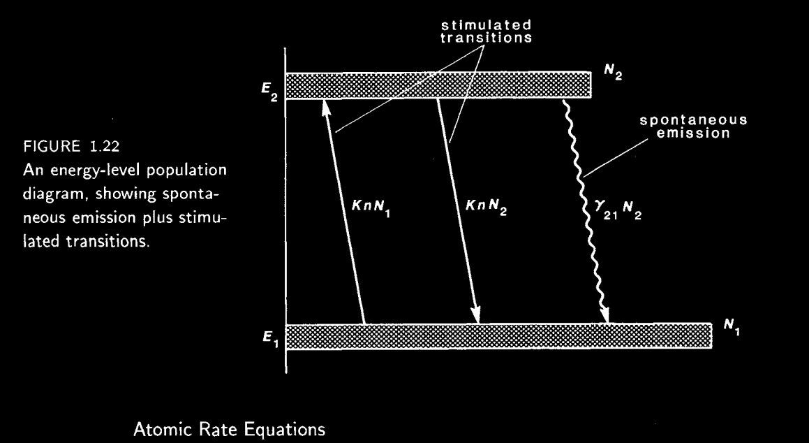
Figure 1.22 from Siegman Lasers Chapter 1.3

Laser Amplification¶

Recall that we can loosely describe the total amount of energy held in the photons as $E_\mathrm{photon} = n(t) \hbar \omega$. This energy can be exchanged with the atoms freely inside the gain medium.

Looking at the Total Rate Equation (7) above, the energy in the signal photons $E_\mathrm{photon}$ changes at the same rate as the number of atoms in the excited state $N_2$. Energy is absorbed from the photons to bump atoms to the excited state, so there must be a minus sign. $E_\mathrm{photon}$ changes as a function of time with the absorption and stimulated emission rate, but the spontaneous emission is irrelevant:

or, equavalently in photon number $n(t)$:

Equation (9) illustrates the importance of population inversion $N_2 > N_1$ for a laser. If $N_2 > N_1$, $n(t)$ will grow exponentially until the populations achieve equilibrium. The photon number $n(t)$ will be maintained by the system indefinitely to maintain energy balance. This gives your laser system an efficient way of giving off its pump energy, and you a way of amplifying a stable, coherent laser.

3.6Coherence and Noise¶

The coherent buildup of stimulated in-phase photon emissions constitutes the fundamentals of a laser.
Coherence refers to how in-phase a laser’s light is: a perfect laser would have the exact same phase for all photons in the beam, while a lightbulb is completely incoherent due to its hot-filament source creating spontaneous emission.

There are two types of coherence: spatial and temporal.

Spatial coherence refers to how uniform the laser phase is over the entire breadth of the beam. The laser phase over space also know as a wavefront, and having a uniform wavefront allows a laser beam to be used as a probe of optical surfaces.

Temporal coherence refers to how uniform the laser phase is over time.
Drifts and noise create differences in laser beam’s power and frequency measured at the same location over time.
We will investigate the different types of noise thoroughly below.

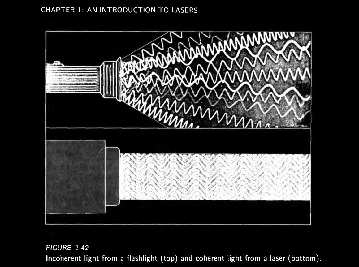
Coherent vs Incoherent light sources: Siegman’s Lasers Chapter 1

We can describe a plane-wave laser amplitude like a complex phasor

where $|E(t)|$ is the amplitude of the wave in units of $\sqrt{\mathrm{W}}$,
$\omega_0$ is the angular frequency, sometimes called the carrier frequency or just carrier, and
$\phi(t)$ is the time-dependent phase of the phasor.

Amplitude noise¶

Amplitude noise $\delta |E(t)|$ directly alters the total coherent power in the electric field. This can come from changes in the pumping power, gain medium, or resonance in the laser oscillator. Amplitude noise is most obvious at the peaks of the sines waves, and cannot be sensed at the sine wave zero crossings.

Phase noise¶

Phase noise $\delta \phi(t)$ alters the phase of the electric field. This can come from fluctuations in the laser oscillator, imperfections in the gain medium, such as thermal fluctuations, or spontaneous emission near to the laser frequency coherently adding with the beam. Phase noise is most obvious at the zero crossings, and less prevalent at the peaks

Below we show some examples of how the amplitude and phase gaussian random noise have different impacts on a sine wave. The noise applied is white noise, meaning that the current sample is totally independent from the next sample i.e. $\phi(t)$ and $\phi(t + \tau)$ have nothing to do with one another.

Frequency Noise¶

Frequency noise is a convenient alternative measure for phase noise. To see this, recall the relationship between phase and frequency in any oscillator:

Any instantaneous change in the phase of our oscillator creates an equivalent change in the frequency of our oscillator.
Using a Laplace transform, we can express this in the frequency domain as

Here it pays to be extra careful about the various terms of $\omega$. The $s$ term is the Laplace parameter, equal to $s = \sigma + i \omega$, representative of the transient $\sigma$ and oscilliatory $\omega$ expression of $\phi$. We can think of the $\omega$ part of the Laplace parameter as a free parameter representing any possible frequency.
$\delta\omega(t)$ are the time-domain fluctuations in the frequency, while
$\delta\omega(s)$ are the frequency-domain fluctuations in the frequency.
In the final line, we have assumed all transient terms $\sigma$ are zero, giving us our final expression of frequency-domain phase noise $\phi(s)$ in terms of frequency-domain frequency noise $\omega(s)$.

What does Eq (12) really mean? Think about the extremes of the equation:
In the low frequency limit, i.e. $\omega \ll 1$, changes in phase $\phi(s)$ have a diminished effect on the frequency $\delta\omega(s)$.
In the high frequency limit, i.e. $\omega \gg 1$, the opposite is true: changes in phase $\phi(s)$ have a large effect on the frequency $\delta\omega(s)$. Fast, sustained changes in the phase $\phi(s)$ will impact our instantaneous frequency $\delta\omega(s)$ more

Intensity Noise¶

Intensity noise, or power noise, is a convenient alternative measure for amplitude noise.
Intensity noise is very simple to measure with a photodiode.

If we imagine our total beam power $P(t)$ is captured by the photodiode, then we can express the power captured $P(t)$ like

The right hand side is the squared amplitude of the incident wave.

This is analogous to quantum mechanics probability calculations using wavefunction amplitudes, and we should not be surprised the same math works for our wave mechanics objects here.

We leave the calculation of intensity noise $\delta P(t)$ as an exercise below.

Coherence Length and Time¶

In the discussion of phase and frequency noise, we assumed we had a carrier oscillator at a constant frequency $\omega_0$, as well as some phase disturbance $\phi(t)$ that can be rewritten as a frequency disturbance $\delta \omega(t)$. Here we will discuss another way to view these disturbances.

In our laser beam, we have an ensemble of $n$ photons, where $n$ is a very large number. These photons are near-but-not-exact copies of each other, co-propagating with nearly the same frequency.

Suppose we have two photons with very close frequencies

Initially, if $\Delta \omega$ is very small, the photons will sum together coherently, yielding our more powerful laser field.

However, after a certain distance traveled together, the frequency difference $\Delta \omega$ starts to decohere our laser beam: we lose our laser beam power because our laser’s individual photons do not have the exact same frequencies. There is no recovering the laser power from decoherence: it leads to the absolute destruction of your coherent beam. The individual photons that make up the beam would have to be picked out and frequency-corrected individually, an impossible task. This is different from beam divergence, for instance, which can be corrected by refocusing a beam.

Suppose we have a laser that emits with a bandwidth, or linewidth, of $\Delta \omega$.
The coherence time $\tau$ is the inverse of that bandwidth:

where $\Delta \omega = 2 \pi \Delta \nu$, and $\Delta \nu$ has units of $\mathrm{Hz}$. This is approximately the length of time the laser can be expected to maintain coherence.

Similarly, the coherence length $L$ is just the space traversed by the laser in the coherence time:

Above we have plotted nine different sine waves with slightly different frequencies $\omega = \omega_0 + \delta\omega(t)$, as well as their sum.
We chose $\nu_0 = 20~\mathrm{Hz}$ and $\delta\omega = 0.5~\mathrm{Hz}$.

On the left hand side, we can see the waves all start out coherently, but this breaks down rapidly.
On the right hand side, the waves are all essentially at random positions.
Although in our example, some total begins to reappear, if we averaged over 100, 1000, or 10²⁰ photons, no average power would be available.

3.7Laser Oscillator¶

A laser oscillator enables repeated exposure of the same laser beam to the gain medium, creating the enormous resonant gain of a laser.
The oscillator enables the complete depletion of the population inversion created by the pump inside the gain medium.

A simple linear standing wave laser oscillator is depicted below.
It is a Fabry-Perot cavity, which consists of two aligned mirrors, with a laser gain material placed in between the mirror.
The mirrors act to “recycle” the laser light back and forth, while the laser gain medium is pumped.

To figure out how much gain we can expect from a laser oscillator in steady state,
we must consider the laser oscillator system and balance losses and gain.
We will learn more about how to model this in the next lecture,
but for now we will consider the open loop gain of the system, which incorporates all laser interactions with the three components: two mirrors, the laser gain medium, and the space between them:

where $g_{rt}$ is the round-trip open loop gain of the laser oscillator,
$r_1$, $r_2$ is the amplitude reflectivity of the mirrors,
$L$ is the total optical length of the laser oscillator,
$L_m$ is the optical length of the laser medium,
$\omega$ is the laser frequency, and
$\alpha_m(\omega) = - \alpha(\omega)$ is the stimulated emission gain based on population inversion from (2).

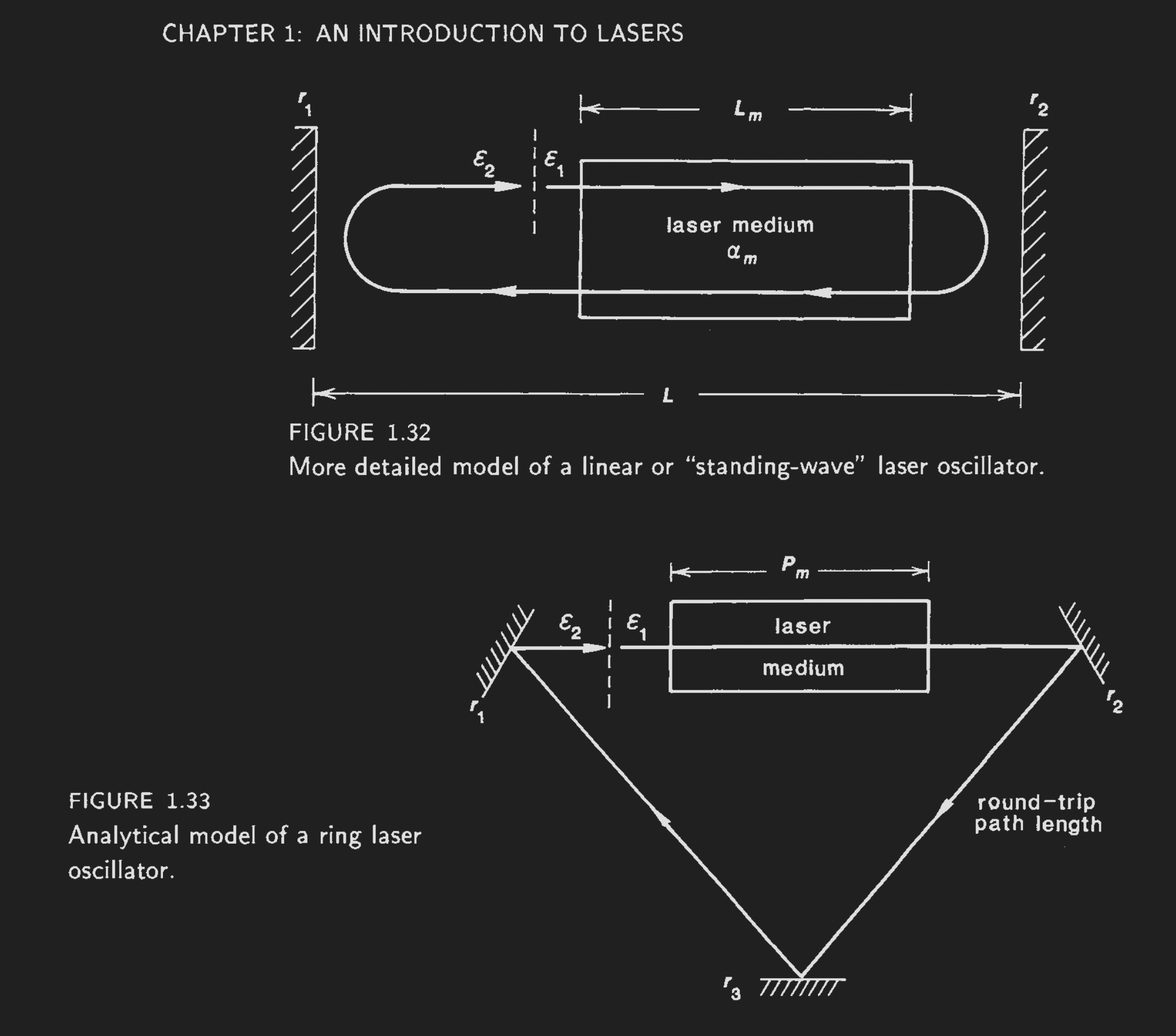Linear “standing wave” laser oscillator and triangular ring laser oscillator.

Initially, a laser starts with a pumped gain medium in a population inversion state. Some outside seed laser, or spontaneous emission, will be emitted into the laser oscillator. If the round-trip gain $\mathrm{Re}(g_{rt}) > 1$, then on each pass, the laser will grow in amplitude. If the round-trip gain $\mathrm{Re}(g_{rt}) < 1$, the laser will die away.

$g_{rt}$ is a complex quantity thanks to the first exponent in (20).
We will simply state for now that $\exp\left( \dfrac{i 2 \omega L}{c} \right) = 1$ to achieve coherent buildup in the laser. Without this condition, all subsequent reflections will be out-of-phase and not coherently summing with one another.

As the laser grows in amplitude, eventually the amplification starts to staturate and cannot go any higher.
Steady-state occurs when

This occurs because the population inversion $\Delta N = N_2 - N_1$ starts to be affected by the large amounts of stimulated emission depleting the $N_2$ state.

The above conditions yields the laser threshold inversion density:

where $R_1 = r_1^2$ and $R_2 = r_2^2$ are the power reflectivity coefficients.

Equation (22) represents the population inversion threshold required to maintain the steady state laser power.
Another interpretation is this is the threshold inversion required in order to achieve any laser oscillation at all.