Light as an Electromagnetic Wave - Lasers and Optomechanics

%matplotlib widget
import numpy as np 
import matplotlib as mpl
import matplotlib.pyplot as plt
from ipywidgets import *

plt.style.use('dark_background')

fontsize = 14
mpl.rcParams.update(
    {
        "text.usetex": False,
        "figure.figsize": (9, 6),
        # "figure.autolayout": True,
        # "font.family": "serif",
        # "font.serif": "georgia",
        # 'mathtext.fontset': 'cm',
        "lines.linewidth": 1.5,
        "font.size": fontsize,
        "xtick.labelsize": fontsize,
        "ytick.labelsize": fontsize,
        "legend.fancybox": True,
        "legend.fontsize": fontsize,
        "legend.framealpha": 0.7,
        "legend.handletextpad": 0.5,
        "legend.labelspacing": 0.2,
        "legend.loc": "best",
        "axes.edgecolor": "#b0b0b0",
        "grid.color": "#707070",  # grid color"
        "xtick.color": "#b0b0b0",
        "ytick.color": "#b0b0b0",
        "savefig.dpi": 80,
        "pdf.compression": 9,
    }
)

1Readings¶

Wikipedia article on Maxwell’s Equations, Solutions in a Vacuum

2What is light?¶

If we are to understand lasers and optomechanics, we must first have a solid grasp of the the nature of light. What is light? is a simple question without a simple answer.

Loosely, light is an excitation in the electromagnetic field which permeates the universe, carrying energy and information that can be directly sensed by the human eye. Humanity’s close relationship with light drove us to study it closely, teaching us first the secrets of electromagnetism, then plunging us into the unintuitive world of quantum mechanics.

2.1The Duality of Light¶

Light is commonly described to be both an electromagnetic wave and particle. This is our way of relating light to waves and particles, two objects humans can easily understand, and sweeping under the rug the complexities. In reality, light is neither a wave nor a particle, but describing light as a complex traveling oscillation in the electromagnetic wave with indeterminant wavelength is not very useful for most people.

A good intuition can be provided by seeing the wave view vs photon view shown in this interactive demo: Electromagnetic Spectrum.

3Electromagnetism: The Wave Equation¶

Maxwell showed that light was an electromagnetic wave, resulting from the interplay of his famous equations in a vacuum (no charges or currents):

\begin{align} \nabla \cdot \boldsymbol{E} &= 0 \end{align}

(1)

\begin{align} \nabla \cdot \boldsymbol{B} &= 0 \end{align}

(2)

\begin{align} \nabla \times \boldsymbol{E} &= - \dfrac{\partial \boldsymbol{B}}{\partial t} \end{align}

(3)

\begin{align} \nabla \times \boldsymbol{B} &= \dfrac{1}{c^2} \dfrac{\partial \boldsymbol{E}}{\partial t} \end{align}

(4)

where $\boldsymbol{E}$ is the electric field vector, $\boldsymbol{B}$ is the magnetic field vector, $\nabla \times$ is a spatial cross-product partial derivative, or curl operator familiar from undergrad E&M, and $c$ is the speed of light.

If we take the curl of the equations in (3):

\begin{align} \nabla \times \nabla \times \boldsymbol{E} &= \nabla \times \left(- \dfrac{\partial \boldsymbol{B}}{\partial t}\right)\\ &= - \dfrac{\partial}{\partial t} \left(\nabla \times \boldsymbol{B} \right) \end{align}

(5)

Subbing in Eq. (4) to the right hand side, and using the curl-of-curl identity

\nabla \times \nabla \times \boldsymbol{E} = \nabla (\nabla \cdot \boldsymbol{E}) - \nabla^2 \boldsymbol{E}

(6)

plus Eq. (1) yields

\begin{align} \nabla^2 \boldsymbol{E} = \dfrac{1}{c^2} \dfrac{\partial^2 \boldsymbol{E} }{\partial t^2} \end{align}

(7)

\begin{align} \nabla^2 \boldsymbol{B} = \dfrac{1}{c^2} \dfrac{\partial^2 \boldsymbol{B} }{\partial t^2} \end{align}

(8)

3.1One-dimensional Plane-wave solution to the wave equation¶

We are going to solve this differential equation in the classic way: by already knowing the answer. This equation is Helmholtz’s equation.

First, we’ll solve Eqs. (7) and (8) in one dimension, and focus on the electric field at first. We can break up electric field

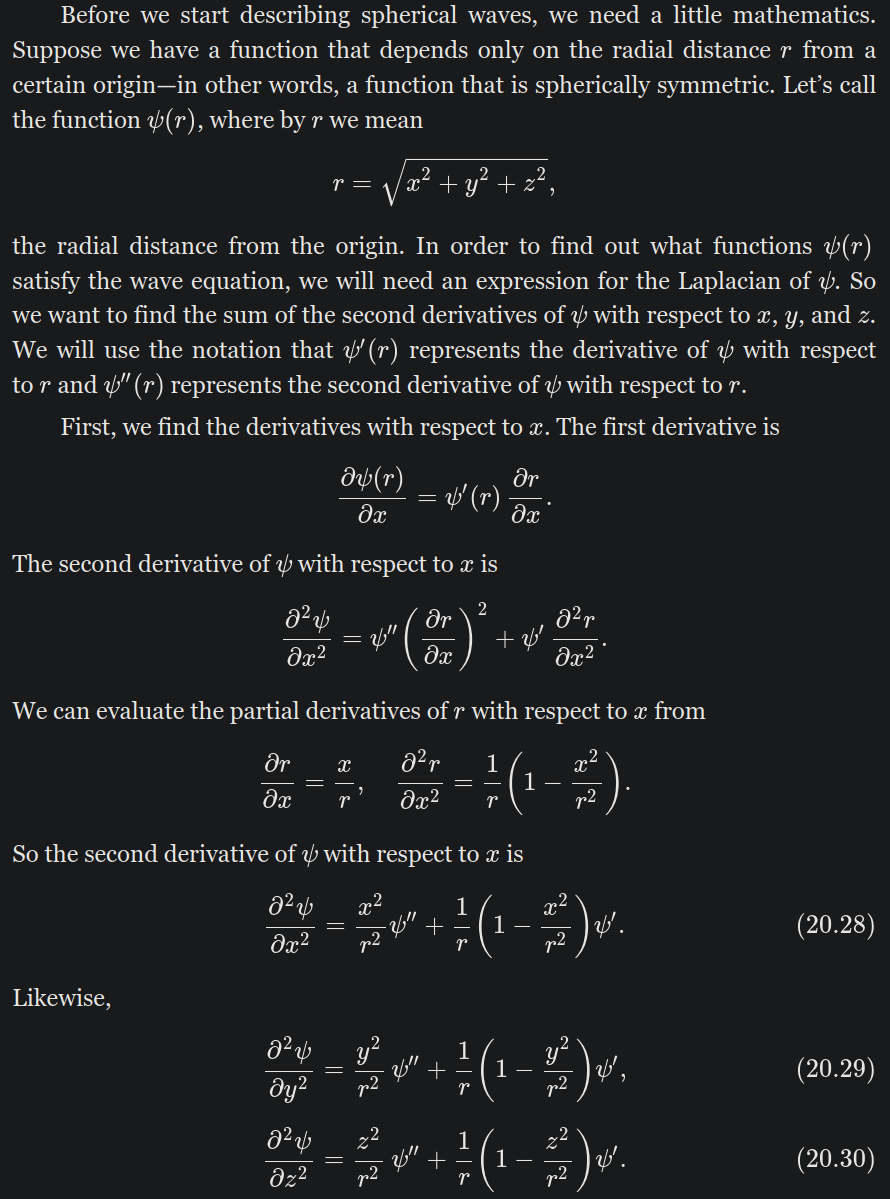
\begin{align} \boldsymbol{E} = (E_x, E_y, E_z) \end{align}

(9)

Recall that the Laplacian

\nabla^2 = \left(\dfrac{\partial^2}{\partial x^2}, \dfrac{\partial^2}{\partial y^2}, \dfrac{\partial^2}{\partial z^2}\right)

(10)

From Gauss’s Law in a vacuum $\nabla \cdot \boldsymbol{E} = 0$ , we know that an electric field cannot propogate in the direction it is pointing. The wave must propogate in a transverse direction.

We will solve for an electric-field in the $x$ -direction $E_x$ that is propogating in the $z$ -direction:

\begin{align} \dfrac{\partial^2 E_x}{\partial z^2} = \dfrac{1}{c^2} \dfrac{\partial^2 E_x }{\partial t^2} \end{align}

(11)

We’ll first employ separation of variables.
We’ll separate the solution for $E_x$ into a pure time and spatial component:

\begin{align} E_x(z,t) = Z(z) T(t) \end{align}

(12)

Applying this separated function

\begin{align} \dfrac{\partial^2 Z}{\partial z^2} T(t) = \dfrac{1}{c^2} \dfrac{\partial^2 T }{\partial t^2} Z(z) \end{align}

(13)

Rearranging:

\begin{align} \dfrac{1}{Z} \dfrac{\partial^2 Z}{\partial z^2} = \dfrac{1}{c^2} \dfrac{1}{T} \dfrac{\partial^2 T }{\partial t^2} \end{align}

(14)

Both sides of Eq. (14) are independent ordinary differential equations, and will equal the same constant.
For convenience later, we will call this constant $-k^2$ .
Then we have

\begin{align} \dfrac{1}{Z} \dfrac{\partial^2 Z}{\partial z^2} = -k^2 \end{align}

(15)

\begin{align} \dfrac{1}{c^2} \dfrac{1}{T} \dfrac{\partial^2 T }{\partial t^2} = -k^2 \end{align}

(16)

We can then offer two oscillating solutions for Eq. (15):

\begin{align} Z(z) = e^{i k z}, \qquad Z(z) = e^{-i k z} \end{align}

(17)

Similarly for Eq. (16), but we define a new constant $\omega = k c$ for simplicity:

\begin{align} T(t) = e^{i \omega t}, \qquad T(t) = e^{-i \omega t} \end{align}

(18)

Combining the above solutions back together using (12) gives us the following general solution:

\begin{align} E_x(z,t) = &A e^{i (k z - \omega t)} + B e^{i (-k z - \omega t)}\\ &C e^{i (k z + \omega t)} + D e^{i (-k z + \omega t)} \end{align}

(19)

with complex coefficients $A,B,C,D$ . The constant $k$ is the wave-number in units of inverse meters,
while the constant $\omega$ is the angular frequency in units of radians / second.

Eq.(19) is generally complex-valued.
However, an electric field must take on a real value, as it is an observable quantity. To reconcile that, our coefficients $A,B,C,D$ must conspire to make $E_x$ real in the end. Most simply, one could set $D = A^*$ and $C = B^*$ , and we’d instantly have

\begin{align} E_x(z,t) = &A' \cos(k z - \omega t + \phi_+) + B' \cos(-k z - \omega t + \phi_-)\\~\\ E_x(z,t) = &\underbrace{A' \cos( k z - \omega t + \phi_+)}_{+z~\text{traveling field}} + \underbrace{B' \cos( -k z - \omega t + \phi_-)}_{-z~\text{traveling field}} \end{align}

(20)

where I’ve assumed the factor of 1/2 into some new $A'$ and $B'$ coefficients, as well as some phases from the complex angles $\phi_{+}$ and $\phi_{-}$ .
We’ve written the solution this way to emphasize that time $t$ always propogates in one direction, but the wave direction $k$ can have either sign.
In this case, $A'$ and $B'$ would be real-valued to maintain a real electric field.

The two components of the $E_x$ solution represent one field propogating in the positive $z$ -direction, and the other field propogating in the negative $z$ -direction.

We mention here that these cosine wave solutions are not the only solutions, but they can be summed into any solution that depends on a variable $u = k z - \omega t$ . See Feynman’s Lecture on Physics Volume II Chapter 20, or Griffith’s Electrodynamics Chapter 9.1.1.

fig = plt.figure()
ax = fig.add_subplot()

amp1 = 1.0
amp2 = 1.0
phase1 = 0.0
phase2 = 0.0
kk = 2 * np.pi * 1
omega = 2 * np.pi * 1
time = 0 

xx = np.linspace(-1.5, 1.5, 1000)
y1 = amp1 * np.cos(kk * xx - omega * time + phase1)
y2 = amp2 * np.cos(-kk * xx - omega * time + phase2)
y3 = y1 + y2

eline1, = ax.plot(xx, y1, label="A' field (+z)")
eline2, = ax.plot(xx, y2, label="B' field (-z)")
eline3, = ax.plot(xx, y3, label="A' + B' field")

ax.set_xlim([xx[0], xx[-1]])
ax.set_ylim([-2, 2])

ax.legend(loc="upper right")
# ax.set_axis_off()
plt.tight_layout()

def update_standing_waves(
    time_slider_value=0, 
    amp1_slider_value=amp1,
    amp2_slider_value=amp2,
    phase1_slider_value=phase1,
    phase2_slider_value=phase2,
):
    """
    Create waves plot with synchronized cosine and sine displays.
    """
    time = time_slider_value
    amp1 = amp1_slider_value
    amp2 = amp2_slider_value
    phase1 = phase1_slider_value
    phase2 = phase2_slider_value
    
    # Calculate sine
    newy1 = amp1 * np.cos(omega * time - kk * xx + phase1)
    newy2 = amp2 * np.cos(omega * time + kk * xx + phase2)
    newy3 = newy1 + newy2

    eline1.set_ydata(newy1)
    eline2.set_ydata(newy2)
    eline3.set_ydata(newy3)
    
    fig.canvas.draw_idle()
    return

# Create interactive widget
time_slider = FloatSlider(
    value=0,
    min=0,
    max=1,
    step=0.01,
    description='time [s]:',
    continuous_update=True,  # Only update on release for better performance
    orientation='horizontal',
    readout=True,
    readout_format='.3f',
)
amp1_slider = FloatSlider(
    value=amp1,
    min=0,
    max=1,
    step=0.01,
    description="A':",
    continuous_update=True,  # Only update on release for better performance
    orientation='horizontal',
    readout=True,
    readout_format='.3f',
)
amp2_slider = FloatSlider(
    value=amp2,
    min=0,
    max=1,
    step=0.01,
    description="B':",
    continuous_update=True,  # Only update on release for better performance
    orientation='horizontal',
    readout=True,
    readout_format='.3f',
)
phase1_slider = FloatSlider(
    value=phase1,
    min=-np.pi,
    max=np.pi,
    step=0.01,
    description=r"$\phi_+$:",
    continuous_update=True,  # Only update on release for better performance
    orientation='horizontal',
    readout=True,
    readout_format='.3f',
)
phase2_slider = FloatSlider(
    value=phase2,
    min=-np.pi,
    max=np.pi,
    step=0.01,
    description=r"$\phi_-$:",
    continuous_update=True,  # Only update on release for better performance
    orientation='horizontal',
    readout=True,
    readout_format='.3f',
)


interact(
    update_standing_waves, 
    time_slider_value=time_slider, 
    amp1_slider_value=amp1_slider,
    amp2_slider_value=amp2_slider,
    phase1_slider_value=phase1_slider,
    phase2_slider_value=phase2_slider
)
plt.show()

Loading...

Accompanying Magnetic Field Plane-Wave Solution¶

Recall that our electric field in the x-direction was

\begin{align*} E_x(z,t) = &A' \cos(k z - \omega t + \phi_+) + B' \cos(-k z - \omega t + \phi_-) \end{align*}

(21)

To get the magnetic field that accompanies Eq. (20), we go back to Faraday’s Law $\nabla \times \boldsymbol{E} = - \dfrac{\partial \boldsymbol{B}}{\partial t}$ .

For $\nabla \times \boldsymbol{E}$ we have (assuming $E_y$ and $E_z = 0$ , and $\phi_+ = \phi_- = 0$ ):

\begin{align} \nabla \times \boldsymbol{E} &= \begin{vmatrix} \boldsymbol{\hat{x}} & \boldsymbol{\hat{y}} & \boldsymbol{\hat{z}}\\[6pt] \dfrac{\partial}{\partial x} & \dfrac{\partial}{\partial y} & \dfrac{\partial}{\partial z} \\[12pt] E_x & E_y & E_z \end{vmatrix} \\ &= \left( \boldsymbol{\hat{y}} \dfrac{\partial}{\partial z} - \boldsymbol{\hat{z}} \dfrac{\partial}{\partial y} \right) E_x\\[1em] &= \boldsymbol{\hat{y}} k \Big[ -A' \sin(k z - \omega t) + B' \sin(- k z - \omega t) \Big] \end{align}

(22)

The above must equal $- \dfrac{\partial \boldsymbol{B}}{\partial t}$ , so we take the antiderivative with respect to time to recover the magnetic field $\boldsymbol{B}$ :

\begin{align} - \dfrac{\partial \boldsymbol{B}}{\partial t} &= \boldsymbol{\hat{y}} k \Big[ -A' \sin(k z - \omega t) + B' \sin(- k z - \omega t) \Big]\\ - \boldsymbol{B} &= \boldsymbol{\hat{y}} k \Bigg[ -\dfrac{1}{\omega} A' \cos(k z - \omega t) + \dfrac{1}{\omega} B' \cos(- k z - \omega t) \Bigg]\\ \rightarrow B_y &= \dfrac{k}{\omega} \Big[ A' \cos(k z - \omega t) - B' \cos(- k z - \omega t) \Big]\\ B_y &= \dfrac{1}{c} \Big[ A' \cos(k z - \omega t) - B' \cos(- k z - \omega t) \Big] \end{align}

(23)

The below Figure Notebook-code shows the electric field alongside the magnetic field, propogating only in one direction.

fig_3d = plt.figure()
ax_3d = fig_3d.add_subplot(projection='3d')

amp = 0.7
kk = 2 * np.pi * 1
omega = 2 * np.pi * 1
time = 0 
x = np.linspace(-2.5, 2.5, 1000)
y = amp * np.sin(omega * time - kk * x)
z = np.zeros_like(x)

eline, = ax_3d.plot(x, z, y, color="#ff9955", label="E-field")
bline, = ax_3d.plot(x, y, z, color="#5599ff", label="B-field")

ax_3d.plot(1.5*x, z, z, lw=0.5, color="white")
ax_3d.plot(z, np.linspace(-2*amp, 2*amp, len(z)), z, lw=0.5, color="white")
ax_3d.plot(z, z, np.linspace(-2*amp, 2*amp, len(z)), lw=0.5, color="white")

ax_3d.set_xlim([x[0], x[-1]])
ax_3d.set_ylim([-1, 1])
ax_3d.set_zlim([-1, 1])
ax_3d.set_aspect('equal')
ax_3d.legend()
ax_3d.set_axis_off()

def update_waves(
    time_slider_value=0, 
    amp_slider_value=0.7
):
    """
    Create waves plot with synchronized cosine and sine displays.
    """
    time = time_slider_value
    amp = amp_slider_value
    
    # Calculate sine
    newy = amp * np.sin(omega * time - kk * x)

    eline.set_data_3d(x, z, newy)
    bline.set_data_3d(x, newy, z)
    # efill = ax_3d.fill_between(x, z, newy, x, z, z, alpha=0.3, color="#ff9955")
    # bfill = ax_3d.fill_between(x, newy, z, x, z, z, alpha=0.3, color="#5599ff")
    
    fig_3d.canvas.draw_idle()
    return

# Create interactive widget
time_slider = FloatSlider(
    value=0,
    min=0,
    max=3,
    step=0.01,
    description='time [s]:',
    continuous_update=True,  # Only update on release for better performance
    orientation='horizontal',
    readout=True,
    readout_format='.3f',
)
amp_slider = FloatSlider(
    value=amp,
    min=0,
    max=1,
    step=0.01,
    description='amplitude:',
    continuous_update=True,  # Only update on release for better performance
    orientation='horizontal',
    readout=True,
    readout_format='.3f',
)

interact(update_waves, time_slider_value=time_slider, amp_slider_value=amp_slider)
plt.show()

Loading...

3.2Generalization in three-dimensions¶

A similar derivation as the plane wave solution above can be performed for $E_y$ and $E_z$ .
We can define a wave-number vector $\mathbf{k} = \left(k_x, k_y, k_z\right)$ and a radial vector $\mathbf{r} = (x, y, z)$ .
Then $\mathbf{k} \cdot \mathbf{r} = k_x x + k_y y + k_z z$ , and we can rewrite the solution in any direction:

\begin{align} \tilde{ \boldsymbol{E} } = \tilde{E_0} e^{i (\mathbf{k} \cdot \mathbf{r} - \omega t)} \hat{n} \end{align}

(24)

where $\hat{n}$ represents the direction the electric field points, and is often called the polarization of the electromagnetic wave.

$\tilde{E_0} = |E_0| e^{i \delta}$ is a constant, and can be complex if the phase term $\delta$ is nonzero.

To get the actual real electric field, the real part of the complex quantity can be taken:

\boldsymbol{E} = \mathrm{Re}(\tilde{ \boldsymbol{E} })

(25)

3.3Spherical Plane Waves¶

Here we introduce the concept of spherical plane waves, following the derivation in Feynman’s Lectures Volume II Chapter 20.

Flat plane waves, like we’ve introduced above, are accurate solutions for continuous sources of single rays of light, or sheets of light propogating in the same direction. However, in some cases point sources serve as the source of our electromagnetic wave, like an oscillating nucleus in a lattice, or a voltage oscillating in an antenna. These point sources correspond to a dipole moment, which emits energy that disperses over 3D space in a nontrivial way.

Here I copy the Feynman lectures derivation of spherical plane waves:

feynman_lecture_volume_2_chapter_20_spherical_wave_excerpt_1.png

feynman_lecture_volume_2_chapter_20_spherical_wave_excerpt_2.png

feynman_lecture_volume_2_chapter_20_spherical_wave_excerpt_3.png

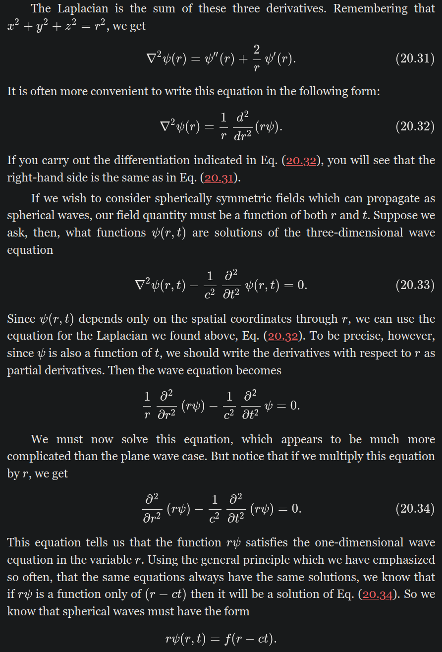
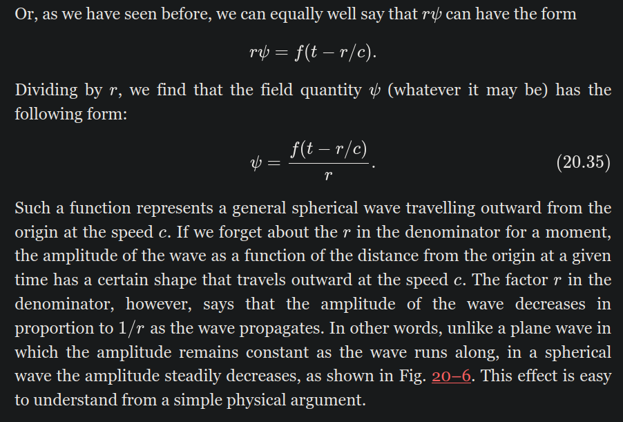
As Feynman states above, The spherical wave amplitude steadily decreases as a function of the distance $r$ . This intuitively makes sense, as the energy from the point source becomes spread out over more space, the amplitude of the wave should decay.

The only minor difference between our plane wave solution above and Feynman’s derivation here is Feynman’s plane wave solution $f(t - r/c)$ is more general than our sinusoidal solutions. Feynman’s solution can represent any arbitrary motion in some medium, like a pulse, so long as it travels along $r$ at a speed $c$

We can reconstruct any pulse or wave propogating along $r$ at a speed $c$ by using some sum of our sinusoids. So, our solutions are valid. The difference between spherical and plane waves can be seen in the two interactive plots below.

# Create figure
fig_2d, axes = plt.subplots(1, 2, figsize=(13, 6))
colormap = 'RdBu_r'

# Create spatial grid
x = np.linspace(-2, 2, 50)
y = np.linspace(-2, 2, 50)
X, Y = np.meshgrid(x, y)

# Wave number
phase = 0
wavelength=1.0
k = 2 * np.pi / wavelength


# Plane wave
Z_plane = np.cos(k * X - phase)

# Spherical wave
R = np.sqrt(X**2 + Y**2)
R = np.where(R < 0.01, 0.01, R)
Z_spherical = np.cos(k * R - phase) / R

# Plane wave
im1 = axes[0].pcolormesh(X, Y, Z_plane, cmap=colormap, 
                         shading='gouraud', vmin=-1, vmax=1)
axes[0].set_xlabel('x', fontsize=12)
axes[0].set_ylabel('y', fontsize=12)
axes[0].set_title(f'Plane Wave (wavelength = {wavelength:.2f})', fontsize=13)
axes[0].set_aspect('equal')
axes[0].grid(True, alpha=0.3)
plt.colorbar(im1, ax=axes[0], label='Amplitude')

# Spherical wave
im2 = axes[1].pcolormesh(X, Y, Z_spherical, cmap=colormap, 
                         shading='gouraud', vmin=-2, vmax=2)
axes[1].set_xlabel('x', fontsize=12)
axes[1].set_ylabel('y', fontsize=12)
axes[1].set_title(f'Spherical Wave (wavelength = {wavelength:.2f})', fontsize=13)
axes[1].set_aspect('equal')
axes[1].grid(True, alpha=0.3)
plt.colorbar(im2, ax=axes[1], label='Amplitude')

plt.tight_layout()
# plt.show()

def plot_both_waves(wavelength=1.0, phase=0.0, colormap='RdBu_r'):
    """
    Plot plane and spherical waves side by side.
    """    
    # Wave number
    new_k = 2 * np.pi / wavelength
    
    # Plane wave
    new_Z_plane = np.cos(new_k * X - phase)
    
    # Spherical wave
    new_Z_spherical = np.cos(new_k * R - phase) / R

    im1.set_array(new_Z_plane.ravel())
    im2.set_array(new_Z_spherical.ravel())

    im1.set_cmap(colormap)
    im2.set_cmap(colormap)

    fig_2d.canvas.draw_idle()
    return

# Interactive widget for side-by-side comparison
interact(plot_both_waves,
         wavelength=FloatSlider(min=0.5, max=3.0, step=0.1, value=1.0,
                               description='Wavelength:',
                               continuous_update=True),
         phase=FloatSlider(min=0, max=2*np.pi, step=0.1, value=0.0,
                          description='Phase (rad):',
                          continuous_update=True),
         colormap=Dropdown(options=['RdBu_r', 'seismic', 'coolwarm', 'viridis', 'plasma'],
                          value='RdBu_r',
                          description='Colormap:')
);
plt.show()

Loading...

fig_1d = plt.figure(figsize=(12, 5))

# Create figure
x = np.linspace(0, 10, 500)
k = 2 * np.pi / wavelength

# Plane wave (constant amplitude)
plane = np.cos(k * x - phase)

# Spherical wave (1/r decay)
x_safe = np.where(x < 0.01, 0.01, x)
spherical = np.cos(k * x - phase) / x_safe

line1, = plt.plot(x, plane, color="#0165fc", linewidth=2, label='Plane Wave')
line2, = plt.plot(x, spherical, 'r-', linewidth=2, label='Spherical Wave (1/r decay)')
line3, = plt.plot(x, 1/x_safe, 'r--', alpha=0.5, linewidth=1, label='1/r envelope')
line4, = plt.plot(x, -1/x_safe, 'r--', alpha=0.5, linewidth=1)

plt.xlabel('Distance from source', fontsize=12)
plt.ylabel('Amplitude', fontsize=12)
plt.title(f'Cross-Section Comparison (wavelength = {wavelength:.2f})', fontsize=13)
plt.grid(True, alpha=0.3)
plt.legend(fontsize=11)
plt.xlim(0, 6)
plt.ylim(-3, 3)
plt.tight_layout()


def plot_cross_section(wavelength=1.0, phase=0.0):
    """
    Plot 1D cross-sections of plane and spherical waves.
    """
    new_k = 2 * np.pi / wavelength
    
    # Plane wave (constant amplitude)
    new_plane = np.cos(new_k * x - phase)
    
    # Spherical wave (1/r decay)
    new_spherical = np.cos(new_k * x - phase) / x_safe
    
    line1.set_ydata(new_plane)
    line2.set_ydata(new_spherical)

    fig_1d.canvas.draw_idle()

# Interactive cross-section plot
interact(plot_cross_section,
         wavelength=FloatSlider(min=0.5, max=3.0, step=0.1, value=1.0,
                               description='Wavelength:',
                               continuous_update=True),
         phase=FloatSlider(min=0, max=2*np.pi, step=0.1, value=0.0,
                          description='Phase (rad):',
                          continuous_update=True));
plt.show()

Loading...

Plane Waves, Lasers, and Wavefronts¶

Here we take a brief step back and consider a laser. A laser is a directed coherent beam of light, and is not well described by plane-wave solutions.

We will find later on that the spherical wave representation is extremely useful for describing lasers propogation close to the axis of propogation. The spherical peaks and troughs form what is called a wavefront, a countour of equal phase forming circles around the point source. More will be said when we discuss lasers and the wave equation solutions using the axial approximation.

3.4Poynting Vectors¶

The following is from Griffith’s Chapter 8.1 In your Electrodynamics class, you should have learned that electric and magnetic fields contain and transport energy and momentum.

The energy stored in the field is just the volume integral $\mathcal{V}$ over the squared fields magnitude:

\begin{align} u = \dfrac{1}{2} \left( \epsilon_0 E^2 + \dfrac{1}{\mu_0} B^2 \right) \end{align}

(26)

where $u$ is the energy density per unit volume, $\epsilon_0$ is the permittivity of free space, $\mu_0$ is the magnetic permeability of free space, and $E^2$ and $B^2$ are the squared electric and magnetic field magnitudes.

The energy radiated away represents the dynamic energy loss over time from our integrated volume. This is described by the Poynting Vector $\boldsymbol{S}$ :

\begin{align} \boxed{ \boldsymbol{S} = \dfrac{1}{\mu_0}(\boldsymbol{E} \times \boldsymbol{B}) } \end{align}

(27)

The Poynting vector $\boldsymbol{S}$ is an energy density flux, and has units of energy per unit time per unit area, or $\mathrm{ \left[ \dfrac{J}{s m^2} \right] = \left[ \dfrac{W}{m^2}\right] }$ where $\mathrm{J}$ is joules and $\mathrm{W}$ is watts. It can be thought of as a way of quantifying energy exchange between energy stored locally in fields and energy radiated away (or toward) the local volume.

Solution to Exercise 1 #

This solution comes from Griffith’s E&M Section 9.2.3:

From our electric and magnetic field wave equation solutions Eqs. (20) and (23), we focus on the field propogating in the $+\hat{z}$ direction, and ignore the phase constant term by setting $\phi_+ = 0$ , letting a magnitude term $E_0 = A'$ .

This gives us our nice phasor expressions:

\begin{align} \boldsymbol{E} &= E_0 \cos(k z - \omega t) \hat{x} \\ \boldsymbol{B} &= \dfrac{ E_0 }{c} \cos(k z - \omega t) \hat{y} \end{align}

(28)

Then the Poynting vector becomes

\begin{align} \boldsymbol{S} &= \dfrac{1}{\mu_0}(\boldsymbol{E} \times \boldsymbol{B}) \\ \boldsymbol{S} &= \dfrac{1}{\mu_0}\left( E_0 \cos(k z - \omega t) \hat{x} \times \dfrac{ E_0 }{c} \cos(k z - \omega t) \hat{y} \right)\\ \boldsymbol{S} &= \dfrac{ E_0^2 }{ c \mu_0 } \cos(k z - \omega t)^2 (\hat{x} \times \hat{y} )\\ \boldsymbol{S} &= c \epsilon_0 E_0^2 \cos(k z - \omega t)^2 \, \hat{z} \end{align}

(29)

where we recall the relation $c^2 = \dfrac{1}{\epsilon_0 \mu_0}$ in the final line. Note that the Poynting vector value oscillates like $\cos(k z - \omega t)^2$ , so the value is sometimes zero and sometimes peaks at $c \epsilon_0 |E_0|^2$ .

The stored energy $u$ in the plane wave relies on $E^2$ and $B^2$ :

\begin{align} E^2 &= E_0^2 \cos(k z - \omega t)^2 \\ B^2 &= \left( \dfrac{ E_0 }{c} \right)^2 \cos(k z - \omega t)^2 \end{align}

(30)

so we have

\begin{align} u &= \dfrac{1}{2} \left( \epsilon_0 E^2 + \dfrac{1}{\mu_0} B^2 \right)\\ u &= \dfrac{1}{2} \left( \epsilon_0 E_0^2 \cos(k z - \omega t)^2 + \dfrac{1}{\mu_0} \left( \dfrac{ E_0 }{c} \right)^2 \cos(k z - \omega t)^2 \right)\\ u &= \epsilon_0 E_0^2 \cos(k z - \omega t)^2 \end{align}

(31)

Note again that for a plane wave, the energy stored in the fields oscillates is sometimes exactly zero.

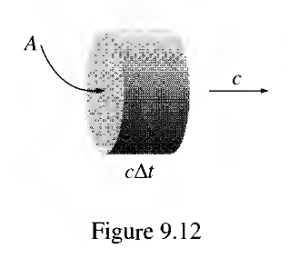
Comparing to Eq. (29) we get the nice relation

\begin{align} \boldsymbol{S} &= c u \hat{z} \end{align}

(32)

In words, this Poynting vector represents the energy transfer of a plane wave through a volume $\mathcal{V}$ over time. The plane wave can be thought of as propogating through some surface with area $A$ at a speed $c$ , and the product $A c$ gives us our volume per unit time. Below is a screenshot from Griffith’s E&M Figure 9.12, illustrating the energy propogation of the plane wave

Intensity¶

The intensity $I$ of light is directly related to the Poynting vector $\boldsymbol{S}$ . It represents the average power per unit area transfered by the light, and can be found simply by taking the average value of the Poynting vector:

\begin{align} I = \langle S \rangle \end{align}

(33)

where $S$ is the magnitude of the Poynting vector $\boldsymbol{S}$ .

As we noted in Exercise 1, the Poynting vector $\boldsymbol{S}$ oscillates like $\cos(k z - \omega t)^2$ for our plane wave solutions, and is sometimes zero and sometimes peaking. The intensity represents the average power transfer over these oscillations.

This is more useful for us, because often relevant electromagnetic oscillations are extremely fast, like in visible lasers with wavelengths on the order of 532 nanometers, the frequency of oscillation is $\nu_\mathrm{green} = 5.64 \times 10^{14}~\mathrm{Hz} = 564~\mathrm{THz}$ .
Humans cannot yet produce electronics to directly analyze light oscillating this fast, so we are relegated to measuring the light’s power, or intensity integrated over the face of a photodiode. Radio waves, on the other hand, can often be directly analyzed, like in the movie Contact (see minute 1:59 here).

Solution to Exercise 2 #

The Poynting vector from (29) is

\begin{align} \boldsymbol{S} &= c \epsilon_0 E_0^2 \cos(k z - \omega t)^2 \, \hat{z} \end{align}

(34)

So the intensity becomes

\begin{align} I &= \left\langle c \epsilon_0 E_0^2 \cos(k z - \omega t)^2 \right\rangle\\ I &= \dfrac{1}{T} \int_0^T c \epsilon_0 E_0^2 \cos(k z - \omega t)^2 dt \end{align}

(35)

where $T$ is the period of one oscillation for our plane wave: $T = \dfrac{1}{\nu} = \dfrac{2 \pi}{\omega}$ .

Here we recall a very convenient integral that we will use very often over this course:

\begin{align} \dfrac{1}{2} = \dfrac{1}{2\pi} \int_0^{2\pi} \cos(\phi)^2 d\phi = \dfrac{1}{2\pi} \int_0^{2\pi} \sin(\phi)^2 d\phi \end{align}

(36)

Essentially, this states that the average integral over one cycle of cosine or sine squared is equal to one half. This is related to the root mean square of an average signal, we’ll explore more in depth later.

We can also state another useful integral:

\begin{align} 0 = \int_0^{2\pi} \cos(\phi) \sin(\phi) d\phi \end{align}

(37)

which represents the orthogonality of $\cos$ and $\sin$ over one cycle.

So, for clarity, I like to redefine our integral Eq. (35) over a phase $\phi(t) = k z - \omega t$ We note that $dt = -\dfrac{d\phi}{\omega}$ , and that $\phi(t = 0) = k z$ and $\phi(t = T) = k z - \omega t = k z - 2 \pi$ . Subbing in all of this yields

\begin{align} I &= \dfrac{\omega}{2\pi} \int_{k z}^{k z - 2 \pi} c \epsilon_0 E_0^2 \cos(\phi)^2 \left(-\dfrac{d\phi}{\omega}\right)\\ I &= -c \epsilon_0 E_0^2 \dfrac{1}{2\pi} \int_{0}^{-2 \pi} \cos(\phi)^2 d\phi \\ I &= c \epsilon_0 E_0^2 \dfrac{1}{2\pi} \int_{0}^{2 \pi} \cos(\phi)^2 d\phi \\ \end{align}

(38)

\boxed{ I = \dfrac{1}{2} c \epsilon_0 E_0^2 }

(39)

This is equation 9.63 from Griffith’s E&M, and represents the plane wave intensity.

Radiation Pressure¶

Radiation pressure represents the momentum-transfer from light electric fields to objects the light touches. Pressure is expressed in terms of force per unit area, and so can be simply related to our intensity value $I$ , which we recall has units of watts per unit area. Remember that power $P = \boldsymbol{F} \cdot \boldsymbol{v}$ , so if we assume $\boldsymbol{v} = c \hat{v}$ , and let $P = I A$ where $A$ is some area, we can write a radiation pressure $p_\mathrm{rad}$ term:

\begin{align} p_\mathrm{rad} = \dfrac{I \cos{\theta} }{c} \end{align}

(40)

where $\theta$ is the angle of incidence of the light on the surface $A$ .

Often, if an entire laser beam’s power $P$ is incident on a surface A, we can divide out that surface and write the radiation pressure force $F_\mathrm{rad}$

\begin{align} F_\mathrm{rad} = \dfrac{P \cos{\theta} }{c} \end{align}

(41)

We note that Equations (40) and (41) are correct for entirely absorbed light. If the light is perfectly reflected, then we get an additional factor of 2 for the momentum change in directions.

3.5Superposition and Interference¶

In a complex world full of electromagnetic waves, superposition offers a simple way of understanding how to calculate the total electric field.
If I have two sources of electric fields $\vec{E_1}, \vec{E_2}$ over the same volume $\mathcal{V}$ ,
then the total electric field $\vec{E}_\mathrm{total}$ is simply their sum:

\begin{align} \vec{E}_\mathrm{total} = \vec{E_1} + \vec{E_2} \end{align}

(42)

Destructive Interference¶

Superposition becomes especially useful for calculating the total intensity $I_\mathrm{total}$ of two plane-wave electric fields incident upon a photodiode:

\begin{align} I_\mathrm{total} &= |\vec{E}_\mathrm{total}|^2\\ &= |\vec{E_1} + \vec{E_2}|^2\\ I_\mathrm{total} &= |\vec{E_1}|^2 + |\vec{E_2}|^2 + \vec{E_1} \cdot \vec{E_2}^* + \vec{E_2} \cdot \vec{E_1}^* \end{align}

(43)

There is a non-trivial interaction between the terms $\vec{E_1}, \vec{E_2}$ in the last line of (43).
If we assume that $\vec{E_2} = \vec{E_1} \exp(i \phi)$ , then (43) becomes

\begin{align} I_\mathrm{total} &= |E_1|^2 + |E_2|^2 + 2 |E_1| |E_2| \cos(\phi) \end{align}

(44)

In this case, some of the expected total intensity $I_\mathrm{total}$ is annihilated via destructive interference.
Not all of the intensity we expected was detected on the photodiode, because the component electric fields were out-of-phase.
If we set $\phi = 0$ , then our fields are exactly in-phase and we recover all of the intensity expected.

Beatnote¶

This interference required both $\vec{E_1}, \vec{E_2}$ to have the same polarization and frequency.
If they had a different frequency $\omega_1$ and $\omega_2$ , then we may get an intensity beatnote, where

\begin{align} I_\mathrm{total} &= |E_1|^2 + |E_2|^2 + 2 |E_1| |E_2| \cos((\omega_1 - \omega_2) t + \phi) \end{align}

(45)

Beatnotes are crucial tools in the world of interferometry.
Typically, we can use one frequency $\omega_1$ as a static reference, also known as a local oscillator.
Then, we can use the second frequency $\omega_2$ as a signal field which acts as a probe, bouncing off some optical element of interest, allowing it to accrue some phase, then combining it back with the local oscillator.
This is known as heterodyne interferometry, and is how your radio works.