Modulations

%matplotlib widget
import numpy as np 
import matplotlib as mpl
import matplotlib.pyplot as plt
from ipywidgets import *

plt.style.use('dark_background')

fontsize = 14
mpl.rcParams.update(
    {
        "text.usetex": False,
        "figure.figsize": (9, 6),
        # "figure.autolayout": True,
        # "font.family": "serif",
        # "font.serif": "georgia",
        # 'mathtext.fontset': 'cm',
        "lines.linewidth": 1.5,
        "font.size": fontsize,
        "xtick.labelsize": fontsize,
        "ytick.labelsize": fontsize,
        "legend.fancybox": True,
        "legend.fontsize": fontsize,
        "legend.framealpha": 0.7,
        "legend.handletextpad": 0.5,
        "legend.labelspacing": 0.2,
        "legend.loc": "best",
        "axes.edgecolor": "#b0b0b0",
        "grid.color": "#707070",  # grid color"
        "xtick.color": "#b0b0b0",
        "ytick.color": "#b0b0b0",
        "savefig.dpi": 80,
        "pdf.compression": 9,
    }
)

In the previous two lectures, we studied two crucial interferometers: the Fabry-Perot and Michelson.
From these basic building blocks, we will eventually build the complex interferometer which is Advanced LIGO.\

However, before we build Advanced LIGO, we need a little more technology.
This tech will revolve around different frequencies of light interacting with our interferometers.
We have already touched on the idea of multiple frequencies at several moments, but now we will formalize it in the form of Scattering Matrices, Transfer Functions, and Modulations.

1Modulations¶

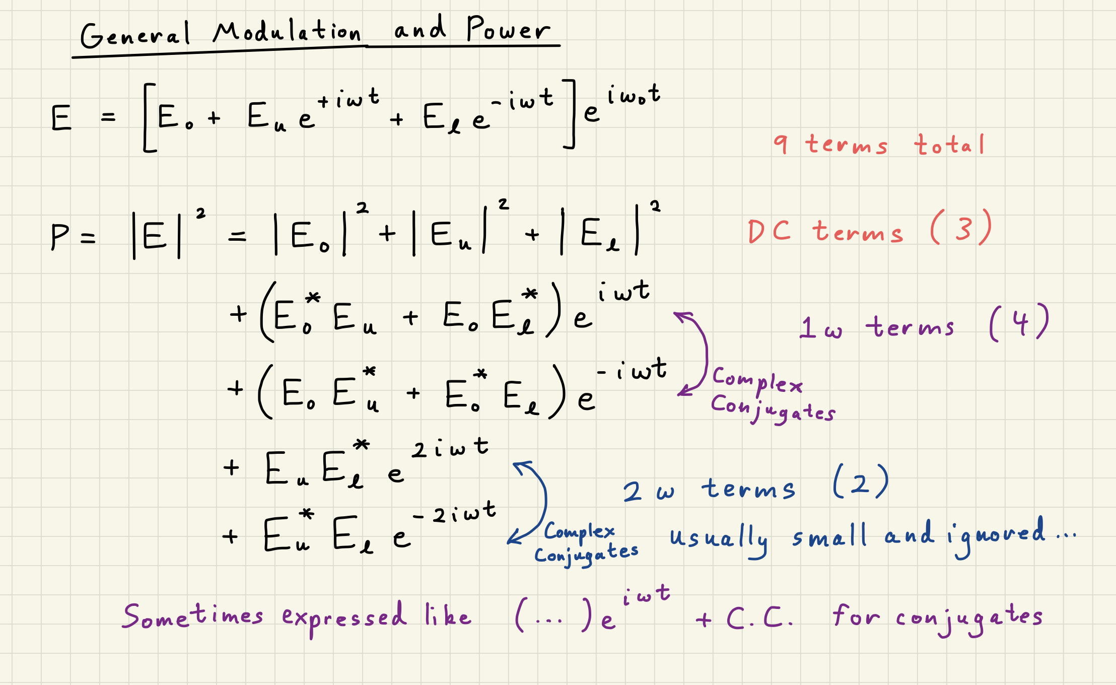
The modulation picture emphasizes the different frequencies of light that are created by different interactions. GWs are detected as infinitesimal modulations applied to highly stabilized laser light. Noise in the laser light, whether quantum or classical, is modulations not caused by GWs.

A perfectly noiseless electric field $E$ is known as the carrier:

\begin{align} E = E_0 e^{i \omega_0 t} \end{align}

(1)

where $\omega_0$ is the carrier frequency, $E_0$ is the carrier amplitude, and $t$ is time.

1.1Phase Modulation¶

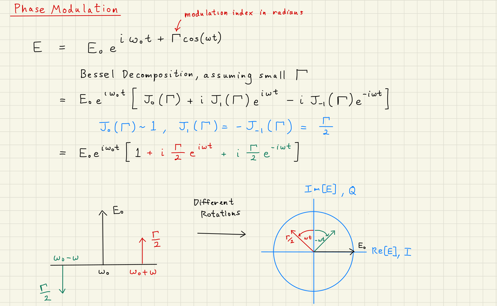
A phase modulation of amplitude $\delta \phi$ at frequency $\omega$ can be applied to the carrier light:

\begin{align} \nonumber E_{\delta \phi} &= E_0 e^{i \phi} \\ E_{\delta \phi} &= E_0 e^{i (\omega_0 t + \delta \phi \cos(\omega t)) } \end{align}

(2)

This can be thought of as splitting the carrier power, which is always a sine wave at $\omega_0$ , off into sidebands at frequencies $\omega_0 \pm \omega$ . Using the Jacobi-Anger expansion on Eq.~(2) yields:

\begin{align} E_{\delta \phi} &= E_0 e^{i \omega_0 t} \displaystyle \sum_{n=-\infty}^{\infty} i^n J_n(\delta \phi) \exp(i n \omega t) \end{align}

(3)

where $J_n$ is the $n^{th}$ Bessel function of the first kind.

If we assume $\delta \phi$ is small, then we can ignore the higher-order sidebands $n \geq 2$ , and write Eq.~(3) as

\begin{align} E_{\delta \phi} &= E_0 e^{i \omega_0 t} \left[ J_0(\delta \phi) + i J_1(\delta \phi) e^{i \omega t} - i J_{-1}(\delta \phi) e^{-i \omega t } \right] \end{align}

(4)

Finally, using $J_{-1}(\delta \phi) = -J_1(\delta \phi)$ , $J_0(\delta \phi) \approx 1$ , and $J_1(\delta \phi) \approx \delta \phi / 2$ , we write the final phase modulation in terms of the carrier $\omega_0$ , upper sideband $\omega_0 + \omega$ and lower sideband $\omega_0 - \omega$ :

\begin{align} E_{\delta \phi} &= E_0 e^{i \omega_0 t} \left( 1 + i \dfrac{\delta \phi}{2} E_0 e^{i \omega t} + i \dfrac{\delta \phi}{2} E_0 e^{-i \omega t} \right)\\ E_{\delta \phi} &= E_0 e^{i \omega_0 t} \left( 1 + i \delta \phi \cos(\omega t) \right) \end{align}

(5)

The key observation of Eq.~(5) is the relative phase of the sidebands compared with the carrier.
The sidebands are aligned with one another when they are orthogonal to the carrier.
Calculating the power in the field,

\begin{align} \nonumber P_{\delta \phi} &= |E_{\delta \phi}|^2 \\ \nonumber &= |E_0|^2 \left(1 + \dfrac{(\delta \phi)^2}{2} + \dfrac{(\delta \phi)^2}{4} \left( e^{i 2 \omega t} + e^{-i 2 \omega t} \right) \right) \\ P_{\delta \phi} &\approx |E_0|^2. \end{align}

(6)

The sidebands push and pull the phase of the carrier by $\delta \phi$ , but to first order do not alter the amplitude. Figure illustrates the sideband and quadrature picture of phase modulation.

Phase Modulation Scheme

Solution to Exercise 1 #

With three terms in the input electric field, multiplied by three terms of the complex conjugate,
we end up with nine total terms in the power expression, which simplifies down to Equation (6):

\begin{align} P_{\delta \phi} &= |E_{\delta \phi}|^2\\ P_{\delta \phi} &= \left[ E_0 e^{i \omega_0 t} \left( 1 + i \dfrac{\delta \phi}{2} E_0 e^{i \omega t} + i \dfrac{\delta \phi}{2} E_0 e^{-i \omega t} \right) \right] \left[ E_0 e^{-i \omega_0 t} \left( 1 - i \dfrac{\delta \phi}{2} E_0 e^{-i \omega t} - i \dfrac{\delta \phi}{2} E_0 e^{i \omega t} \right) \right] \\ P_{\delta \phi} &= |E_0|^2 \left[ 1 + \dfrac{(\delta \phi)^2}{4} + \dfrac{(\delta \phi)^2}{4} - i \dfrac{\delta \phi}{2} E_0 e^{-i \omega t} - i \dfrac{\delta \phi}{2} E_0 e^{i \omega t} + i \dfrac{\delta \phi}{2} E_0 e^{i \omega t} + i \dfrac{\delta \phi}{2} E_0 e^{-i \omega t} + \dfrac{(\delta \phi)^2}{4} e^{i 2 \omega t} + \dfrac{(\delta \phi)^2}{4} e^{-i 2 \omega t} \right]\\ P_{\delta \phi} &= |E_0|^2 \left(1 + \dfrac{(\delta \phi)^2}{2} + \dfrac{(\delta \phi)^2}{4} \left( e^{i 2 \omega t} + e^{-i 2 \omega t} \right) \right) \end{align}

(7)

Note we still have our $2\omega$ power oscillation here.

Adding in the second order terms in $J_0 = 1 - \dfrac{\Gamma^2}{4}$ helps us avoid “adding power” to final term, but does not completely eliminate our issue.

\begin{align} E_{\delta \phi} &= E_0 e^{i \omega_0 t} \left( \left(1 - \dfrac{(\delta \phi)^2}{4} \right) + i \dfrac{\delta \phi}{2} E_0 e^{i \omega t} + i \dfrac{\delta \phi}{2} E_0 e^{-i \omega t} \right) \\ \rightarrow P_{\delta \phi} &= |E_0|^2 \left(1 + \dfrac{(\delta \phi)^4}{16} + \dfrac{(\delta \phi)^2}{4} \left( e^{i 2 \omega t} + e^{-i 2 \omega t} \right) \right) \end{align}

(8)

Integrating the right hand side over one period of the $2\omega$ oscillation eliminates the exponetial terms, yielding

\begin{align} \dfrac{1}{2\pi} \int_0^{2\pi} P_{\delta \phi} d(2 \omega t) = |E_0|^2 \left( 1 + \dfrac{(\delta \phi)^4}{16} \right) \end{align}

(9)

which is pretty good power conservation for small $\delta \phi$ .

1.2Frequency noise¶

Frequency noise is mathematically equivalent to a phase modulation. Using the definition of frequency as the time derivative of phase, $d\phi/dt$ , and the phase $\phi$ from Eq.(2), we calculate the relationship between frequency noise and phase modulation \cite{HeinzelThesis}:

\begin{align} \nonumber \dfrac{d\phi}{dt} &= \dfrac{d}{dt}(\omega_0 t + \delta \phi \cos(\omega t)) \\ \dfrac{d\phi}{dt} &= \omega_0 - \omega \delta \phi \sin(\omega t) \end{align}

(10)

The frequency can be broken down into the carrier term $\omega_0$ and the noise term $\delta \nu$ , where

\begin{align} \dfrac{2 \pi \delta \nu}{\omega} = \delta \phi \end{align}

(11)

where $\delta \nu$ is the amplitude of the frequency swing.

We can substitute Eq.(11) into Eq.(5) with no change in the final result (except an arbitrary phase advance of $\pi/2$ for both sidebands):

\begin{align} E_{\delta \nu} &= E_0 e^{i \omega_0 t} \left( 1 - \dfrac{\pi \delta \nu}{\omega} e^{i \omega t} + \dfrac{\pi \delta \nu}{\omega} e^{-i \omega t} \right) \end{align}

(12)

Here we recall the distinction between $\omega_0$ , $\omega$ , and $\delta \omega$ . The carrier frequency is $\omega_0$ , this is a constant, $\omega_0 = 2 \pi c / \lambda = 1.77 \times 10^{15}~\mathrm{rad/s}$ (The Advanced LIGO laser wavelength $\lambda = 1064~\mathrm{nm}$ ). The modulation frequency itself is $\omega$ , this is how fast the carrier frequency changes. The frequency modulation amplitude $\delta \nu$ is how much the carrier frequency changes.

1.3Amplitude modulation¶

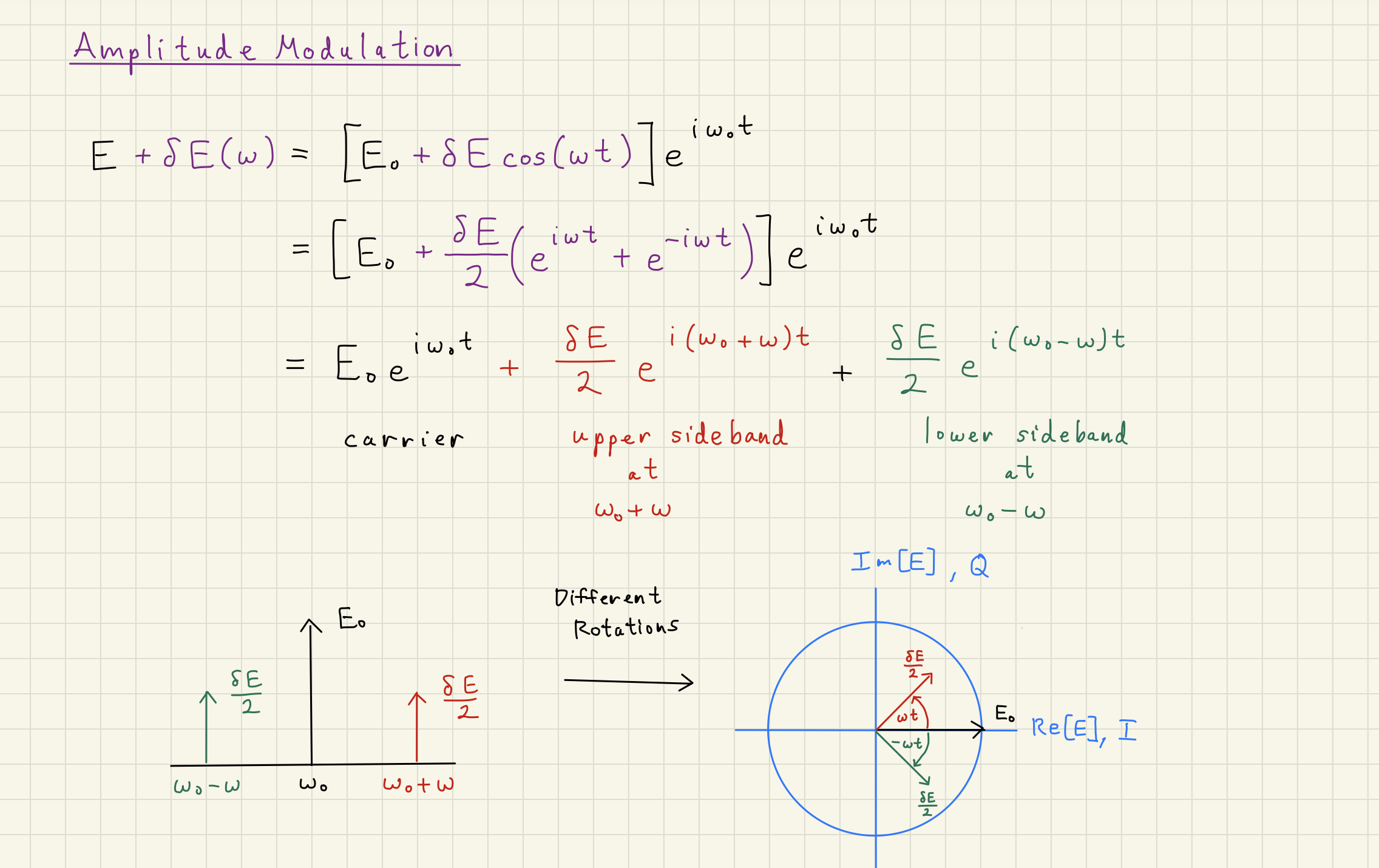
An amplitude modulation of amplitude $\delta E$ at frequency $\omega$ can be applied to the carrier light:

\begin{align} \nonumber E_{\delta E} &= E_0 e^{i \omega_0 t} \left( 1 + \dfrac{\delta E}{E_0} \cos(\omega t) \right) \\ E_{\delta E} &= E_0 e^{i \omega_0 t} \left( 1 + \dfrac{\delta E}{2 E_0} e^{i \omega t} + \dfrac{\delta E}{2 E_0} e^{-i \omega t} \right) \end{align}

(13)

Again, the key observation of Eq.(13) is the relative phase of the sidebands compared with the carrier. This time, the sidebands are aligned with one another when they are also aligned with the carrier. Calculating the power in the field,

\begin{align} \nonumber P_{\delta E} &= |E_{\delta E}|^2 \\ \nonumber &= |E_0|^2 \left(1 + \dfrac{2 \delta E}{E_0} \cos(\omega t) + \dfrac{(\delta E)^2}{E_0^2} \cos(\omega t)^2 \right) \\ P_{\delta E} &\approx P_0 \left(1 + \dfrac{2 \delta E}{E_0} \cos(\omega t) \right). \end{align}

(14)

The sidebands push and pull the amplitude of the carrier by $\delta E$ , but do not alter the phase. Figure illustrates the sideband and quadrature picture of amplitude modulation.

Amplitude Modulation Scheme

1.4Intensity noise¶

Relative intensity noise (RIN) is mathematically equivalent to amplitude modulation. From Eq.(14), we can relate relative intensity noise to relative amplitude noise (RAN). Dividing Eq.(14) by $P_0$ , we define the relative intensity noise in terms of amplitude modulation:

\begin{align} \dfrac{\delta P}{P_0} &= \dfrac{2 \delta E}{E_0} \end{align}

(15)

Going back to the expression for amplitude modulation $E_{\delta E}$ Eq.(13), we can express the electric field $E_{\delta P}$ and power $P_{\delta E}$ in terms of relative intensity noise $\delta P / P$ :

\begin{align} E_{\delta P} &= E_0 e^{i \omega_0 t} \left( 1 + \dfrac{\delta P}{4 P_0} e^{i \omega t} + \dfrac{\delta P}{4 P_0} e^{-i \omega t} \right)\\ P_{\delta E} &= P_0 \left(1 + \dfrac{\delta P}{P_0} \cos(\omega t) \right) \end{align}

(16)

def carrier(phi, mod_depth):
    return (1 - mod_depth**2 / 4) * np.exp(1j * phi)

def upper_phase_sideband(phi, theta, mod_depth):
    return 1j * mod_depth / 2 * np.exp(1j * (theta + phi))
    
def lower_phase_sideband(phi, theta, mod_depth):
    return 1j * mod_depth / 2 * np.exp(-1j * (theta - phi))

def upper_amp_sideband(phi, theta, mod_depth):
    return mod_depth / 2 * np.exp(1j * (theta + phi))
    
def lower_amp_sideband(phi, theta, mod_depth):
    return mod_depth / 2 * np.exp(-1j * (theta - phi))

fig1 = plt.figure(figsize=(12,8))
ax1 = fig1.add_subplot()

phis = np.linspace(-np.pi, np.pi, 100)

phi0 = 0
theta0 = 0
mod_depth = 0.5

# Arc
plot_carriers = carrier(phis, mod_depth)

plot_carriers_real = np.real(plot_carriers)
plot_carriers_imag = np.imag(plot_carriers)

# Vectors
plot_carrier = carrier(phi0, mod_depth)
plot_usb = upper_amp_sideband(phi0, theta0, mod_depth)
plot_lsb = lower_amp_sideband(phi0, theta0, mod_depth)
plot_total = plot_carrier + plot_usb + plot_lsb

plot_carrier_real = np.real(plot_carrier)
plot_carrier_imag = np.imag(plot_carrier)
plot_usb_real = np.real(plot_usb)
plot_usb_imag = np.imag(plot_usb)
plot_lsb_real = np.real(plot_lsb)
plot_lsb_imag = np.imag(plot_lsb)
plot_total_real = np.real(plot_total)
plot_total_imag = np.imag(plot_total)

arc1, = ax1.plot(plot_carriers_real, plot_carriers_imag, label="Carrier Phasor")
# line1, = ax1.plot([0, plot_carrier_real], [0, plot_carrier_imag], 'o-', label="Carrier")
# line2, = ax1.plot([0, plot_usb_real], [0, plot_usb_imag], 'o-', label="Upper Sideband")
# line3, = ax1.plot([0, plot_lsb_real], [0, plot_lsb_imag], 'o-', label="Lower Sideband")
# line4, = ax1.plot([0, plot_total_real], [0, plot_total_imag], 'o-', label="Total Electric Field")

arrow1 = ax1.arrow(0, 0, plot_carrier_real, plot_carrier_imag, shape='full', color="C1", lw=2, 
                  length_includes_head=True, head_width=.025, zorder=2, label="Carrier")
arrow2 = ax1.arrow(0, 0, plot_usb_real, plot_usb_imag, shape='full', color="C2", lw=2, 
                  length_includes_head=True, head_width=.025, zorder=2, label="Upper Sideband")
arrow3 = ax1.arrow(0, 0, plot_lsb_real, plot_lsb_imag, shape='full', color="C3", lw=2, 
                  length_includes_head=True, head_width=.025, zorder=2, label="Lower Sideband")
arrow4 = ax1.arrow(0, 0, plot_total_real, plot_total_imag, shape='full', color="C4", lw=2, 
                  length_includes_head=True, head_width=.025, zorder=2, label="Total Electric Field")
arrow5 = ax1.arrow(plot_carrier_real, plot_carrier_imag, plot_usb_real, plot_usb_imag, shape='full', color="C2", lw=2, 
                  length_includes_head=True, head_width=.025, zorder=2, label="Upper Sideband")
arrow6 = ax1.arrow(plot_carrier_real+plot_usb_real, plot_carrier_imag+plot_usb_imag, plot_lsb_real, plot_lsb_imag, shape='full', color="C3", lw=2, 
                  length_includes_head=True, head_width=.025, zorder=2, label="Lower Sideband")

ax1.set_xlabel("Real")
ax1.set_ylabel("Imaginary $i$")
ax1.set_xlim([-1.5, 1.5])
ax1.set_ylim([-1.5, 1.5])
ax1.grid()

ax1.set_title("Amplitude Modulation")

ax1.legend(bbox_to_anchor=(1.01, 0.6))
ax1.set_aspect('equal')
# plt.tight_layout()

def update_amplitude_modulation(
    phi0_slider_value=phi0,
    theta0_slider_value=theta0,
    mod_depth_slider_value=mod_depth
):
    """
    Create waves plot with synchronized cosine and sine displays.
    """
    new_phi0 = np.pi / 180 * phi0_slider_value
    new_theta0 = np.pi / 180 * theta0_slider_value
    new_mod_depth = mod_depth_slider_value
    
    # Arc
    new_plot_carriers = carrier(phis, new_mod_depth)
    
    new_plot_carriers_real = np.real(new_plot_carriers)
    new_plot_carriers_imag = np.imag(new_plot_carriers)
    
    # Vectors
    new_plot_carrier = carrier(new_phi0, new_mod_depth)
    new_plot_usb = upper_amp_sideband(new_phi0, new_theta0, new_mod_depth)
    new_plot_lsb = lower_amp_sideband(new_phi0, new_theta0, new_mod_depth)
    new_plot_total = new_plot_carrier + new_plot_usb + new_plot_lsb
    
    new_plot_carrier_real = np.real(new_plot_carrier)
    new_plot_carrier_imag = np.imag(new_plot_carrier)
    new_plot_usb_real = np.real(new_plot_usb)
    new_plot_usb_imag = np.imag(new_plot_usb)
    new_plot_lsb_real = np.real(new_plot_lsb)
    new_plot_lsb_imag = np.imag(new_plot_lsb)
    new_plot_total_real = np.real(new_plot_total)
    new_plot_total_imag = np.imag(new_plot_total)

    # line1.set_xdata(new_xx0)
    # line1.set_ydata(new_yy0)
    arc1.set_xdata(new_plot_carriers_real)
    arc1.set_ydata(new_plot_carriers_imag)
    arrow1.set_data(x=0, y=0, dx=new_plot_carrier_real, dy=new_plot_carrier_imag)
    arrow2.set_data(x=0, y=0, dx=new_plot_usb_real, dy=new_plot_usb_imag)
    arrow3.set_data(x=0, y=0, dx=new_plot_lsb_real, dy=new_plot_lsb_imag)
    arrow4.set_data(x=0, y=0, dx=new_plot_total_real, dy=new_plot_total_imag)
    arrow5.set_data(x=new_plot_carrier_real, y=new_plot_carrier_imag, dx=new_plot_usb_real, dy=new_plot_usb_imag)
    arrow6.set_data(x=new_plot_carrier_real+new_plot_usb_real, y=new_plot_carrier_imag+new_plot_usb_imag, dx=new_plot_lsb_real, dy=new_plot_lsb_imag)

    # ax1.set_title(r"$(r, \theta)$ = " + f"({new_plot_rr0:.3f}, {180/np.pi*new_plot_theta0:.3f}"+r"$^\circ$)")
    
    fig1.canvas.draw_idle()
    return

# Create interactive widget
phi0_slider1 = FloatSlider(
    value=phi0,
    min=0,
    max=180,
    step=0.1,
    description=r"$\phi_0$ [deg]:",
    continuous_update=True,  # Only update on release for better performance
    orientation='horizontal',
    readout=True,
    readout_format='.3f',
)
theta0_slider1 = FloatSlider(
    value=theta0,
    min=0,
    max=360,
    step=0.1,
    description=r"$\omega t$ [deg]:",
    continuous_update=True,  # Only update on release for better performance
    orientation='horizontal',
    readout=True,
    readout_format='.3f',
)
mod_depth_slider1 = FloatSlider(
    value=mod_depth,
    min=0,
    max=1,
    step=0.01,
    description=r"$\Gamma$:",
    continuous_update=True,  # Only update on release for better performance
    orientation='horizontal',
    readout=True,
    readout_format='.3f',
)

interact(
    update_amplitude_modulation,
    phi0_slider_value=phi0_slider1,
    theta0_slider_value=theta0_slider1,
    mod_depth_slider_value=mod_depth_slider1,
)
plt.show()

Loading...

fig2 = plt.figure(figsize=(12,8))
ax2 = fig2.add_subplot()

phis = np.linspace(-np.pi, np.pi, 100)

phi0 = 0
theta0 = 0
mod_depth = 0.5

# Arc
plot_carriers = carrier(phis, mod_depth)

plot_carriers_real = np.real(plot_carriers)
plot_carriers_imag = np.imag(plot_carriers)

# Vectors
plot_carrier = carrier(phi0, mod_depth)
plot_usb = upper_phase_sideband(phi0, theta0, mod_depth)
plot_lsb = lower_phase_sideband(phi0, theta0, mod_depth)
plot_total = plot_carrier + plot_usb + plot_lsb

plot_carrier_real = np.real(plot_carrier)
plot_carrier_imag = np.imag(plot_carrier)
plot_usb_real = np.real(plot_usb)
plot_usb_imag = np.imag(plot_usb)
plot_lsb_real = np.real(plot_lsb)
plot_lsb_imag = np.imag(plot_lsb)
plot_total_real = np.real(plot_total)
plot_total_imag = np.imag(plot_total)

arc12, = ax2.plot(plot_carriers_real, plot_carriers_imag, label="Carrier Phasor")
# line1, = ax2.plot([0, plot_carrier_real], [0, plot_carrier_imag], 'o-', label="Carrier")
# line2, = ax2.plot([0, plot_usb_real], [0, plot_usb_imag], 'o-', label="Upper Sideband")
# line3, = ax2.plot([0, plot_lsb_real], [0, plot_lsb_imag], 'o-', label="Lower Sideband")
# line4, = ax2.plot([0, plot_total_real], [0, plot_total_imag], 'o-', label="Total Electric Field")

arrow12 = ax2.arrow(0, 0, plot_carrier_real, plot_carrier_imag, shape='full', color="C1", lw=2, 
                  length_includes_head=True, head_width=.025, zorder=2, label="Carrier")
arrow22 = ax2.arrow(0, 0, plot_usb_real, plot_usb_imag, shape='full', color="C2", lw=2, 
                  length_includes_head=True, head_width=.025, zorder=2, label="Upper Sideband")
arrow32 = ax2.arrow(0, 0, plot_lsb_real, plot_lsb_imag, shape='full', color="C3", lw=2, 
                  length_includes_head=True, head_width=.025, zorder=2, label="Lower Sideband")
arrow42 = ax2.arrow(0, 0, plot_total_real, plot_total_imag, shape='full', color="C4", lw=2, 
                  length_includes_head=True, head_width=.025, zorder=2, label="Total Electric Field")

arrow52 = ax2.arrow(plot_carrier_real, plot_carrier_imag, plot_usb_real, plot_usb_imag, shape='full', color="C2", lw=2, 
                  length_includes_head=True, head_width=.025, zorder=2, label="Upper Sideband")
arrow62 = ax2.arrow(plot_carrier_real+plot_usb_real, plot_carrier_imag+plot_usb_imag, plot_lsb_real, plot_lsb_imag, shape='full', color="C3", lw=2, 
                  length_includes_head=True, head_width=.025, zorder=2, label="Lower Sideband")

ax2.set_xlabel("Real")
ax2.set_ylabel("Imaginary $i$")
ax2.set_xlim([-1.5, 1.5])
ax2.set_ylim([-1.5, 1.5])
ax2.grid()

ax2.set_title("Phase Modulation")

ax2.legend(bbox_to_anchor=(1.01, 0.6))
ax2.set_aspect('equal')
# plt.tight_layout()

def update_phase_modulation(
    phi0_slider_value=phi0,
    theta0_slider_value=theta0,
    mod_depth_slider_value=mod_depth
):
    """
    Create waves plot with synchronized cosine and sine displays.
    """
    new_phi0 = np.pi / 180 * phi0_slider_value
    new_theta0 = np.pi / 180 * theta0_slider_value
    new_mod_depth = mod_depth_slider_value
    
    # Arc
    new_plot_carriers = carrier(phis, new_mod_depth)
    
    new_plot_carriers_real = np.real(new_plot_carriers)
    new_plot_carriers_imag = np.imag(new_plot_carriers)
    
    # Vectors
    new_plot_carrier = carrier(new_phi0, new_mod_depth)
    new_plot_usb = upper_phase_sideband(new_phi0, new_theta0, new_mod_depth)
    new_plot_lsb = lower_phase_sideband(new_phi0, new_theta0, new_mod_depth)
    new_plot_total = new_plot_carrier + new_plot_usb + new_plot_lsb
    
    new_plot_carrier_real = np.real(new_plot_carrier)
    new_plot_carrier_imag = np.imag(new_plot_carrier)
    new_plot_usb_real = np.real(new_plot_usb)
    new_plot_usb_imag = np.imag(new_plot_usb)
    new_plot_lsb_real = np.real(new_plot_lsb)
    new_plot_lsb_imag = np.imag(new_plot_lsb)
    new_plot_total_real = np.real(new_plot_total)
    new_plot_total_imag = np.imag(new_plot_total)

    # line1.set_xdata(new_xx0)
    # line1.set_ydata(new_yy0)
    arc12.set_xdata(new_plot_carriers_real)
    arc12.set_ydata(new_plot_carriers_imag)
    arrow12.set_data(x=0, y=0, dx=new_plot_carrier_real, dy=new_plot_carrier_imag)
    arrow22.set_data(x=0, y=0, dx=new_plot_usb_real, dy=new_plot_usb_imag)
    arrow32.set_data(x=0, y=0, dx=new_plot_lsb_real, dy=new_plot_lsb_imag)
    arrow42.set_data(x=0, y=0, dx=new_plot_total_real, dy=new_plot_total_imag)
    arrow52.set_data(x=new_plot_carrier_real, y=new_plot_carrier_imag, dx=new_plot_usb_real, dy=new_plot_usb_imag)
    arrow62.set_data(x=new_plot_carrier_real+new_plot_usb_real, y=new_plot_carrier_imag+new_plot_usb_imag, dx=new_plot_lsb_real, dy=new_plot_lsb_imag)

    # ax2.set_title(r"$(r, \theta)$ = " + f"({new_plot_rr0:.3f}, {180/np.pi*new_plot_theta0:.3f}"+r"$^\circ$)")
    
    fig2.canvas.draw_idle()
    return

# Create interactive widget
phi0_slider2 = FloatSlider(
    value=phi0,
    min=0,
    max=180,
    step=0.1,
    description=r"$\phi_0$ [deg]:",
    continuous_update=True,  # Only update on release for better performance
    orientation='horizontal',
    readout=True,
    readout_format='.3f',
)
theta0_slider2 = FloatSlider(
    value=theta0,
    min=0,
    max=360,
    step=0.1,
    description=r"$\omega t$ [deg]:",
    continuous_update=True,  # Only update on release for better performance
    orientation='horizontal',
    readout=True,
    readout_format='.3f',
)
mod_depth_slider2 = FloatSlider(
    value=mod_depth,
    min=0,
    max=1,
    step=0.01,
    description=r"$\Gamma$:",
    continuous_update=True,  # Only update on release for better performance
    orientation='horizontal',
    readout=True,
    readout_format='.3f',
)

interact(
    update_phase_modulation,
    phi0_slider_value=phi0_slider2,
    theta0_slider_value=theta0_slider2,
    mod_depth_slider_value=mod_depth_slider2,
)
plt.show()

Loading...

1.5Modulation Scattering Matrices¶

Recall that a scattering matrix $\boldsymbol{S}$ is a generalized way of describing the interaction of several input electric fields $\vec{E}_\mathrm{in}$ to several output electric fields $\vec{E}_\mathrm{out}$ :

\vec{E}_\mathrm{out} = \boldsymbol{S} \vec{E}_\mathrm{in}

(17)

We can harness the power of scattering matrices to describe electric fields with different frequencies $\omega$ , like those created in phase or amplitude modulations.

For instance, recall the phase modulation electric field picture from (5):

\begin{align} E_{\delta \phi} &= E_0 e^{i \omega_0 t} \left( 1 + i \dfrac{\delta \phi}{2} e^{i \omega t} + i \dfrac{\delta \phi}{2} e^{-i \omega t} \right) \end{align}

(18)

In the above equation, we have sideband electric fields created by some phase modulation process with modulation depth $\delta \phi$ and modulation frequency $\omega$ .

The input was just the raw carrier field $E_0 e^{i \omega_0 t}$ .
The output is the carrier field, still oscillating at $\omega_0$ , and unchanged in magnitude to first order, represented by the leading 1 in the parentheses.
The upper and lower sidebands, on the other hand, are no longer oscillating at $\omega_0$ , but are oscillating at $\omega_0 + \omega$ for the upper and $\omega_0 - \omega$ for the lower:

\begin{alignat}{3} \text{Carrier:} \quad E_\mathrm{carrier} &= E_0 e^{i \omega_0 t}\\ \text{Upper Sideband:} \quad E_\mathrm{usb} &= i \dfrac{\delta \phi}{2} E_0 e^{i (\omega_0 + \omega) t}\\ \text{Lower Sideband:} \quad E_\mathrm{lsb} &= i \dfrac{\delta \phi}{2} E_0 e^{i (\omega_0 - \omega) t} \end{alignat}

(19)

In this case, we can write a $3 \times 1$ scattering matrix to describe phase modulation:

\begin{align} \begin{bmatrix} E_\mathrm{carrier} \\ E_\mathrm{usb} \\ E_\mathrm{lsb} \end{bmatrix} = \begin{bmatrix} 1 \\ i \dfrac{\delta \phi}{2} e^{i \omega t} \\ i \dfrac{\delta \phi}{2} e^{-i \omega t} \end{bmatrix} \begin{bmatrix} E_0 e^{i \omega_0 t} \end{bmatrix} \end{align}

(20)

1.6Relationship between Real and Imaginary quadrature and Amplitude and Phase quadrature¶

Here we dive into a general topic of quadrature definitions. There are many names for our quadratures:

Real and Imaginary
Amplitude and Phase
Cosine and Sine

What exactly do each of these represent?
What is important is that our electric field phasors require two real numbers to fully describe them.
We harness the power of complex numbers to represent the fields, and those always assume a real and imaginary basis.

However, when we start to describe the superposition of several electric fields,
the Amplitude and Phase quadrature start to become more useful, especially in these sideband modulation pictures.

What is crucial about modulations, or changes in an electric field in general, is what the modulation or change is relative to.
The carrier field typically serves as this reference.
The carrier is just a phasor, described as

E_0 e^{i \omega_0 t}

(21)

where $E_0$ is the amplitude and $\omega_0$ is the frequency of the carrier.

When we look at the modulation equations above (5) or (13), they are relative to the carrier phasor.
In other words, the sidebands rotate with the carrier, always changing their direction of modulation relative to the carrier.
This makes sense, because the sidebands were generated as frequency offsets from the carrier.

When we analyze general modulations on a light field, and want to describe how those modulations are affecting the field, it is convention to put the carrier light in the cosine quadrature for analysis:

E(t) = [E_0 + E_1(t)] \cos(\omega_0 t) + E_2(t) \sin(\omega_0 t)

(22)

where $E_1(t)$ are the amplitude fluctuations, and $E_2(t)$ are the phase fluctuations.

So this convention defines the relationship between amplitude and phase quadratures and cosine and sine quadrutures.

Noise and Squeezed Light Picture¶

When we think about noise on light, these can readily be described in terms of amplitude and phase modulations.

The ultimate limit for noise on light is quantum fluctuations in the electric field.
Those are usually represented as an uncertainty ball around the carrier phasor, shown below.

Squeezing is the reallocation of noise from one quadrature to another.
That is represented by the squeezing of the uncertainty ball, usually in the phase or amplitude quadratures.
This produces the “ball-and-stick” picture shown below.

The actual effect on the light measured is shown in the sine-wave oscillations seen below.

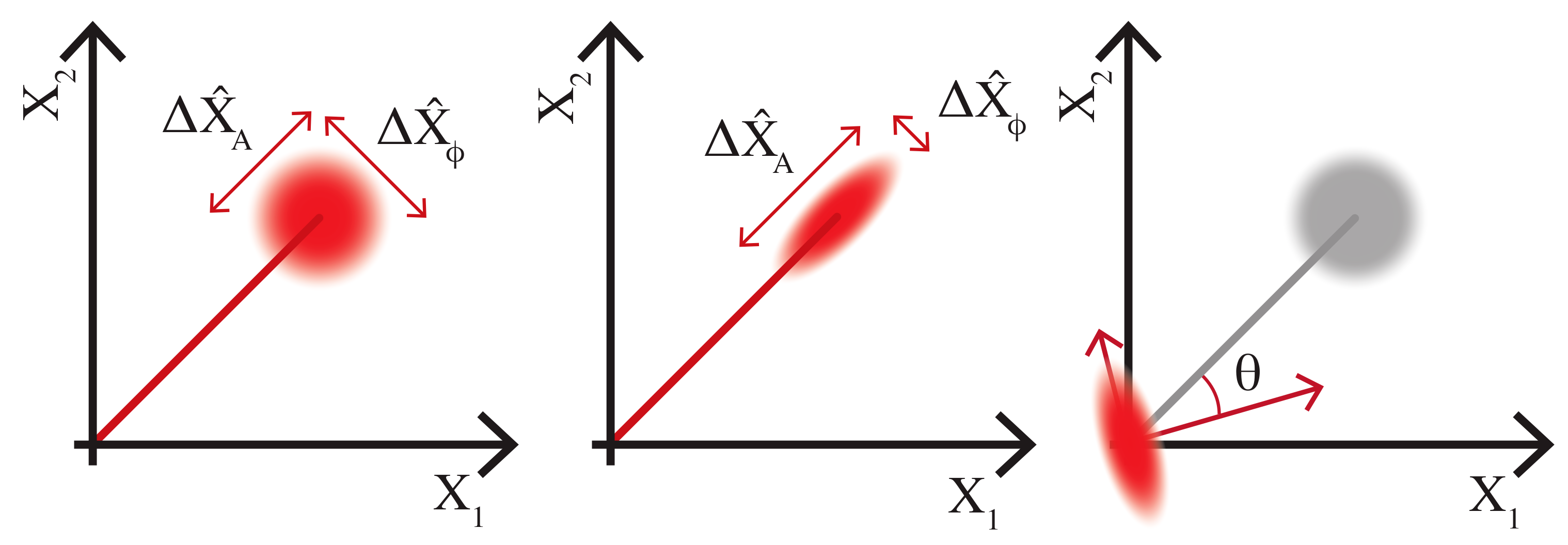
Figure from Dwyer, Mansell, McCuller Squeezing in Gravitational Wave Detectors

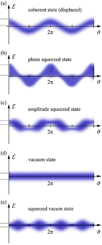
Figure from Wikipedia on Squeezed States of Light

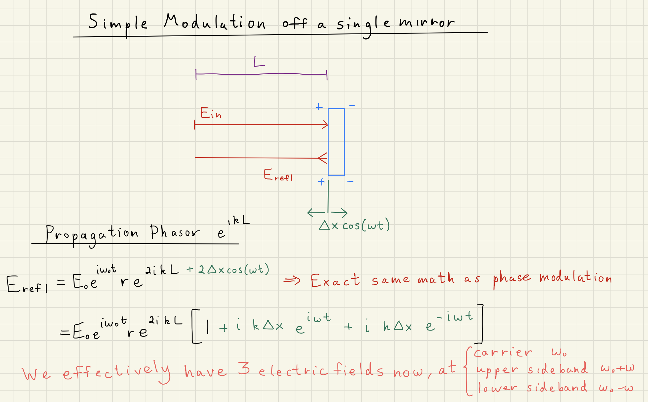
1.7Modulation of a reflection off a mirror¶

Now, we want to relate the above modulations to a real system.
Suppose we have a mirror oscillating at a frequency $\omega$ with a small amplitude $\Delta x$ .
An electric field $E_\mathrm{in} = E_0 e^{i \omega_0 t}$ is incident on that mirror over a propogation distance $L$ .
What is the total reflected electric field $E_\mathrm{refl}$ ?

The below diagram illustrates the above situation.
We have the incident electric field on the mirror:

\begin{align} E_\mathrm{inc} = E_\mathrm{in} e^{i k (L + \Delta x \cos(\omega t))} \end{align}

(23)

and the electric field reflected off and traveling back along that distance again:

\begin{align} E_\mathrm{refl} &= E_\mathrm{in} e^{i 2 k (L + \Delta x \cos(\omega t))}\\ E_\mathrm{refl} &= E_0 e^{i \omega_0 t} e^{i 2 k L} e^{i 2 k \Delta x \cos(\omega t)} \end{align}

(24)

Looking at Equation (2), we can identify the similarities between it and Eq. (24) above.
In short, our phase modulation term $\delta \phi = 2 k \Delta x$ , where the 2 comes from the double-pass through the length modulation $\Delta x$ .
Following the same Jacobi-Anger math as above, we can write Eq. (24) as

\begin{align} &= E_0 e^{i \omega_0 t} e^{i 2 k L} \left(1 + i k \Delta x e^{i \omega t} + i k \Delta x e^{-i \omega t} \right) \end{align}

(25)

Now we have three electric fields from our initial single carrier: carrier still at $\omega_0$ , but some sidebands at $\omega_0 \pm \omega$ .
For mirror reflections, normally $\omega$ will be in the audio frequencies of 10 - 10000 kHz, but in general could be any frequency.

Mirror Reflection Phase Modulation

1.8Review of Modulations¶

The key to all of the modulations above are the creation of the additional phasors at $\omega_0 + \omega$ and $\omega_0 - \omega$ .
These represent entirely different frequencies of light.

Typically, $\omega_0$ is the carrier frequency, which is a huge number, on the 100 terrahertz scale.
$\omega$ is either in the audio band of 10 - 10000 Hz or radio-frequency band of a few megahertz. So, the frequencies are fairly close in absolute terms (100 THz ± 10 MHz is a fairly small difference.) This helps us understand how the light carrier and sidebands interact with optical elements in a similar way.

Modulations can be created by specific interactions of the laser carrier with optical elements, including power or frequency fluctuations from the laser, thermal fluctuations of the mirror surface, “popsical” modes of mirror mounts, or seismic motion of a suspended mirror.
Anything that interacts with the laser imposes some modulations upon it, but these can be measured and controlled.

1.9Modulations in the Quadrature Picture¶

Amplitude and phase quadratures offer a convenient way of representing light. Instead of upper and lower sidebands, modulations are broken down into how they affect the carrier.

The quadrature operators can be written as a vector $\vec{E}$ representing the modulations of the total electric field:

\begin{align} \vec{E} = \begin{pmatrix} E_1 \\ E_2 \end{pmatrix}. \end{align}

(26)

where $E_1$ is the amplitude quadrature and $E_2$ is the phase quadrature.

This representation is a bit different than our previous quadrature representation of the real (cosine) and imaginary (sine) quadratures.
This amplitude and phase quadrature representation can be well-motivated by Carlton Caves two photon formalism. While I won’t go into this here, quantum optics textbooks, and several LIGO papers and theses give a nice overview of the two photon formalism relationship between the sideband and quadrature picture.

We can express the sideband amplitude and phase modulations from (16) and (12) in quadrature representation using (26).

We break up the total electric field $\vec{E}_{tot} = \vec{E} + \vec{e}(\omega)$ into a ``static’’ component $\vec{E}$ centered around the carrier frequency $\omega_0$ and a modulation, or Fourier, component $\vec{e}(\omega)$ at the relative signal frequencies $\omega_0 \pm \omega$ . Expressing an electric field modulated in both intensity and frequency $\vec{E}_{tot}$ from Eqs (16) and (12) in quadrature representation yields

\begin{align} \vec{E}_{tot} &= \vec{E} + \vec{e}(\omega) \\ \vec{E} &= E_0 e^{i \omega_0 t} \begin{pmatrix} 1 \\ 0 \end{pmatrix} \\ \vec{e}(\omega) &= E_0 e^{i \omega_0 t} e^{i \omega t} \Bigg[ \dfrac{2 \pi \delta \nu}{\omega} \begin{pmatrix} 0 \\ 1 \end{pmatrix} + \dfrac{\delta P}{2 P} \begin{pmatrix} 1 \\ 0 \end{pmatrix} \Bigg] \end{align}

(27)

Here, we add our upper and lower sidebands from Eqs.~(16) and (12) together to produce the quadrature scalers.

For example, we recover intensity noise from Eq.~(16). Let $\delta \nu \rightarrow 0$ for $\vec{e}(\omega)$ in Eq.~(27), and take the dot product of $\vec{E}_{tot}$ with itself to get power $P_{\delta P}$ :

\begin{align} \nonumber P_{\delta P} &= \left| \vec{E} + \vec{e}(\omega) \right|^2 \\ \nonumber &= \left| \vec{E} \right|^2 + \vec{E}^* \cdot \vec{e}(\omega) + \vec{E} \cdot \vec{e}^*(\omega) + \left|\vec{e}(\omega)\right|^2 \\ \nonumber &\approx E_0^2 \left( 1 + \dfrac{\delta P}{2 P} e^{i \omega t} + \dfrac{\delta P}{2 P} e^{-i \omega t} \right) \begin{pmatrix} 1 & 0 \end{pmatrix} \cdot \begin{pmatrix} 1 \\ 0 \end{pmatrix} \\ P_{\delta P} &= P_0 \left( 1 + \dfrac{\delta P}{P} \cos(\omega t) \right) \end{align}

(28)

The result from Eq.~(28) matches Eq.~(16).

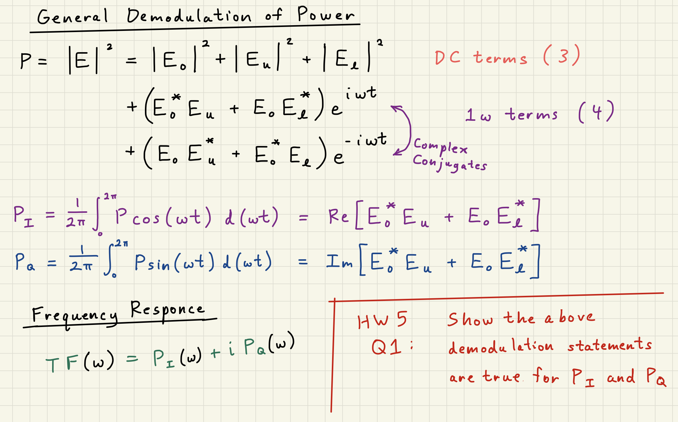
2Demodulations¶

Above, we’ve been calculating the effects of modulations on electric fields and power quantities for phase and amplitude modulations.
Some of the information we’ll care about for interferometers, especially relative lengths, will be caught up in the beatnote between our carrier frequency $\omega_0$ and sideband frequency $\omega_0 \pm \omega$ .
Demodulation is the process of extracting that information.

Demodulation is simply the process of integrating a power signal over one cycle of the frequency of interest.
So if I have some power signal $P(t)$ and I care about the signal at frequency $\omega$ , I would integrate over one full $2\pi$ cycle of $\omega$ :

\begin{align} P_\mathrm{DC} &= \dfrac{1}{2 \pi} \int_0^{2\pi} P(t) d(\omega t)\\ P_I &= \dfrac{1}{2 \pi} \int_0^{2\pi} P(t) \cos(\omega t) d(\omega t)\\ P_Q &= \dfrac{1}{2 \pi} \int_0^{2\pi} P(t) \sin(\omega t) d(\omega t)\\ \end{align}

(29)

where $P_\mathrm{DC}$ is the constant DC power on the diode, and $P_I$ and $P_Q$ are the power signals measured in the I-quadrature (cosine quadrature) and Q-quadrature (sine quadrature). Normally demodulations are written as an integral over all time $t$ , but if the power signal is stationary the power signals should remain the same over one cycle $\omega t \in [0, 2\pi]$ .

Basically, what Eq. (29) allows us to “pick-out” the signals of the total electric field quadratures incident on the photodiode at the beatnote frequency $\omega$ .
Imagine that the time signal $P(t) = 2 P_I \cos(\omega t) + 2 P_Q \sin(\omega t)$ .
When we multiply by $\cos(\omega t)$ , we get

P(t) \cos(\omega t) = 2 P_I \cos^2(\omega t) + 2 P_Q \sin(\omega t)\cos(\omega t)

(30)

Integrating the above over one cycle of $\omega t$ will give

\dfrac{1}{2 \pi} \int_0^{2\pi} \cos^2(\omega t) d(\omega t) = \dfrac{1}{2}\\~\\ \dfrac{1}{2 \pi} \int_0^{2\pi} \sin(\omega t) \cos(\omega t) d(\omega t) = 0

(31)

so we’d get the constant $P_I$ out of that integral.
Multiplying by $\sin(\omega t)$ similarly picks out $P_Q$ .

In this way, demodulation allows us to reconstruct the total electric field incident on a photodetector, simply by measuring the power signal $P(t)$ and comparing it to some oscillator at $\omega$ .
This can be an incredibly powerful tool, as we will see when we study Pound-Drever-Hall laser locking.

2.1General Modulation and Demodulation¶

Screenshot 2026-01-24 at 12.04.54 AM.png

General modulation terms

Screenshot 2026-01-24 at 12.06.43 AM.png

General demodulation

2.2Example: Length Estimation using two frequencies of light¶

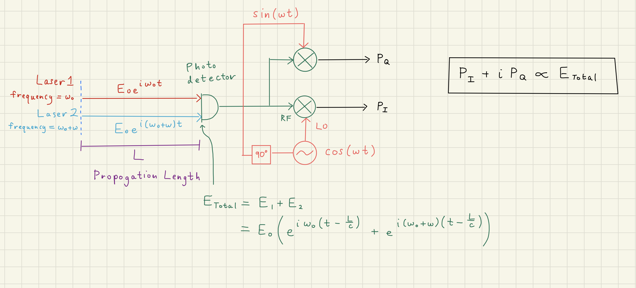
Screenshot 2026-01-24 at 10.26.13 PM.png

Solution to Exercise 2 #

First, our input phasors for our lasers light will be

\begin{align*} E_{in1} &= |E_1|e^{i \omega_0 t}\\ E_{in2} &= |E_2|e^{i (\omega_0 + \omega) t} \end{align*}

(32)

and after the propogate a distance $L$ , they will have accrued a different phase $\phi_i = - k_i L$ , where $k_1 = \omega_0 / c$ and $k_2 = (\omega_0 + \omega) / c$ :

\begin{align*} E_1 &= E_{in1} e^{-i k_1 L} = |E_1|e^{i \omega_0 t} e^{-i \omega_0 L / c}\\ E_2 &= E_{in2} e^{-i k_2 L} = |E_2|e^{i (\omega_0 + \omega) t} e^{-i (\omega_0 + \omega) L / c} \end{align*}

(33)

The total electric field is

\begin{align*} E_\mathrm{total} &= E_1 + E_2\\ E_\mathrm{total} &= |E_1|e^{i \omega_0 t} e^{-i \omega_0 L / c} + |E_2|e^{i (\omega_0 + \omega) t} e^{-i (\omega_0 + \omega) L / c}\\ E_\mathrm{total} &= e^{i \omega_0 (t - L / c)} ( |E_1| + |E_2|e^{i \omega (t - L / c)} ) \end{align*}

(34)

where in the last line we factor out the common phasor $e^{i \omega_0 (t - L / c)}$ .

The total power is

\begin{align*} P_\mathrm{total} &= |E_1 + E_2|^2\\ P_\mathrm{total} &= \left(e^{i \omega_0 (t - L / c)} ( |E_1| + |E_2|e^{i \omega (t - L / c)} ) \right) \left( e^{-i \omega_0 (t - L / c)} ( |E_1| + |E_2|e^{-i \omega (t - L / c)} ) \right)\\ P_\mathrm{total} &= \left( |E_1| + |E_2|e^{i \omega (t - L / c)} \right) \left( |E_1| + |E_2|e^{-i \omega (t - L / c)} \right)\\ P_\mathrm{total} &= |E_1|^2 + |E_2|^2 + 2 |E_1||E_2|\cos \left[ \omega \left(t - \dfrac{L}{c} \right) \right] \end{align*}

(35)

Then, our demodulation integrals become

\begin{align} P_\mathrm{DC} &= \dfrac{1}{2 \pi} \int_0^{2\pi} P_\mathrm{total} d(\omega t) \\ P_\mathrm{DC} &= |E_1|^2 + |E_2|^2\\~\\ P_I &= \dfrac{1}{2 \pi} \int_0^{2\pi} P_\mathrm{total} \cos(\omega t) d(\omega t) \\ P_I &= |E_1| |E_2| \cos\left[ \dfrac{L \omega}{c} \right] \\~\\ P_Q &= \dfrac{1}{2 \pi} \int_0^{2\pi} P_\mathrm{total} \sin(\omega t) d(\omega t) \\ P_Q &= |E_1| |E_2| \sin\left[ \dfrac{L \omega}{c} \right] \\ \end{align}

(36)

remember that $\cos(A + B) = \cos(A) \cos(B) - \sin(A) \sin(B)$

These results points to a clear way of reconstructing $P_\mathrm{total}$ , as well as isolating $L$ .
We can get our complex phasor $P_\mathrm{total}$ back by looking at $P_I + i P_Q$ :

\begin{align} P_I + i P_Q = |E_1| |E_2| \exp\left[ i \dfrac{L \omega}{c} \right] \end{align}

(37)

which is the non-time-dependent part of the beatnote term of $P_\mathrm{total}$ .\

By finding the argument $\theta$ of $P_I + i P_Q$ , that will be equal to $\dfrac{L \omega}{c}$ . If we know the frequency $\omega$ , we can estimate $L$ :

L = \dfrac{c}{\omega} \arg[P_I + i P_Q]

(38)

The issue arises from phase-wrapping: if $\dfrac{L \omega}{c} > 2\pi$ , we’ll underestimate $L$ .
One can alter $\omega$ to make $\dfrac{L \omega}{c} < 2\pi$ , or use other methods to find the correct order-of-magnetude for $L$ that makes sense.

2.3Homodyne Detection¶

Suppose we have an interesting signal we would like to detect from some optical system, like the small vibration of a mirror in a Michelson interferometer corresponding to gravitational wave motion.
Unfortunately, that mirror motion produces a phase modulation for us

Homodyne detection is a crucial concept for understanding the self-demodulation of laser signal incident on a photodetector.

Homodyne Angle $\zeta$ ¶

The \textit{homodyne angle} $\zeta$ is the static angle between the carrier phase and the signal sideband basis. The homodyne angle controls what mixed quadrature $a_\zeta$ is measured on the photodetector \cite{KLMTV, Harms2003, GerryKnight2004, Enomoto2016}:

\begin{align} a_\zeta = a_1 \cos \zeta + a_2 \sin \zeta \end{align}

(39)

In the sideband picture, the total electric field can be written

\begin{align} E_{tot} = E_0 e^{i \omega_0 t} \left[ e^{i \zeta} + \dfrac{\delta_+}{2} e^{i \omega t} + \dfrac{\delta_-}{2} e^{-i \omega t} \right] \end{align}

(40)

where $\delta_+, \delta_-$ is some arbitrary complex modulation.

\begin{figure}[hbt!] \centering \includegraphics[width=\textwidth]{./chapters/modulations/figures/homodyne_angle_diagram.pdf} \caption[Homodyne angle diagram]{ Diagram (a) illustrates a local oscillator $\vec{L}$ beating with a signal sideband $\vec{a}$ with homodyne angle $\zeta$ . Diagram (b) is a phasor diagram illustrating the homodyne angle. In this diagram, $\vec{a}$ is entirely in $a_2$ , so the homodyne angle must be adjusted to $\zeta = \pi/2$ or $\zeta = 3\pi/2$ . } \label{fig:homodyne_angle} \end{figure}

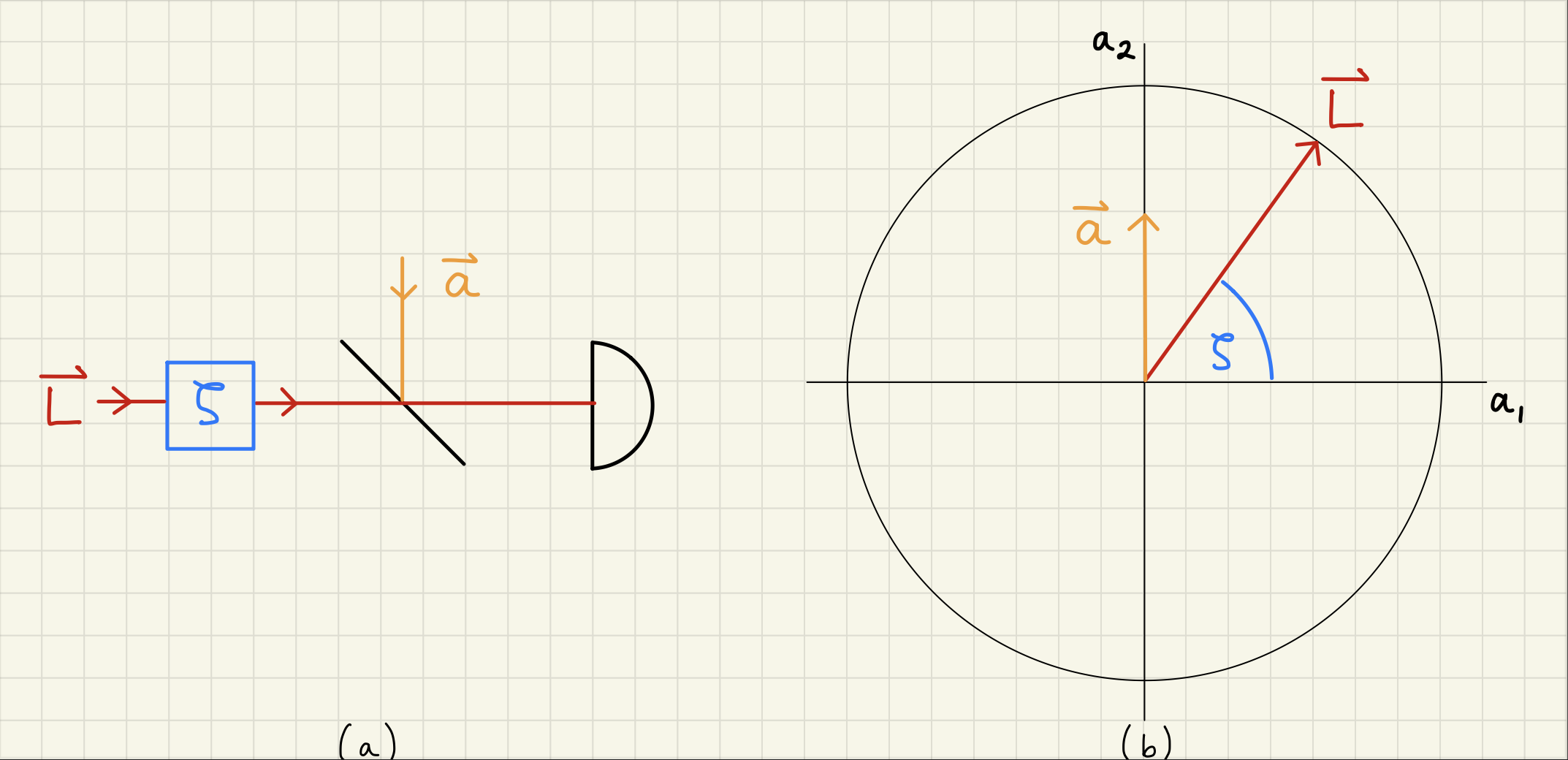
Screenshot 2026-02-03 at 11.44.26 PM.png

Figure~\ref{fig:homodyne_angle} shows a basic example of homodyne detection, with local oscillator carrier $\vec{L}$ and sidebands $\vec{a}$ . The local oscillator phase can be adjusted by the homodyne angle

\begin{align} \vec{L} = E_0 e^{i \omega_0 t} e^{i \zeta} \end{align}

(41)

In terms of the total electric field and total power oscillations, using the quadrature representation,

\begin{align} \vec{E}_{tot} &= \dfrac{1}{\sqrt{2}} \left( \vec{L} + \vec{a} \right) \\ \nonumber P_{tot} &= \dfrac{1}{2} \left| \vec{L} + \vec{a} \right|^2 \\ \nonumber P_{tot} &= \dfrac{1}{2} \left| \vec{L} \right|^2 + \vec{L} \cdot \vec{a} \\ \nonumber P_{tot} &= \dfrac{1}{2} \left| \vec{L} \right|^2 + E_0 \begin{pmatrix} \cos \zeta & \sin \zeta \end{pmatrix} \begin{pmatrix} a_1 \\ a_2 \end{pmatrix} \\ \nonumber P_{tot} &= \dfrac{1}{2} E_0^2 + E_0 a_\zeta \\ P_{tot} &= \dfrac{1}{2} P_0 + P_\zeta \end{align}

(42)

Suppose that $\vec{a}$ is in $a_2$ , as in Figure~\ref{fig:homodyne_angle}. Then the detected power oscillations at $P_\zeta$ is:

\begin{align} P_\zeta = E_0 a_2 \sin \zeta \end{align}

(43)

and we can detect the phase modulation when the homodyne angle $\zeta = \pi/2$ .