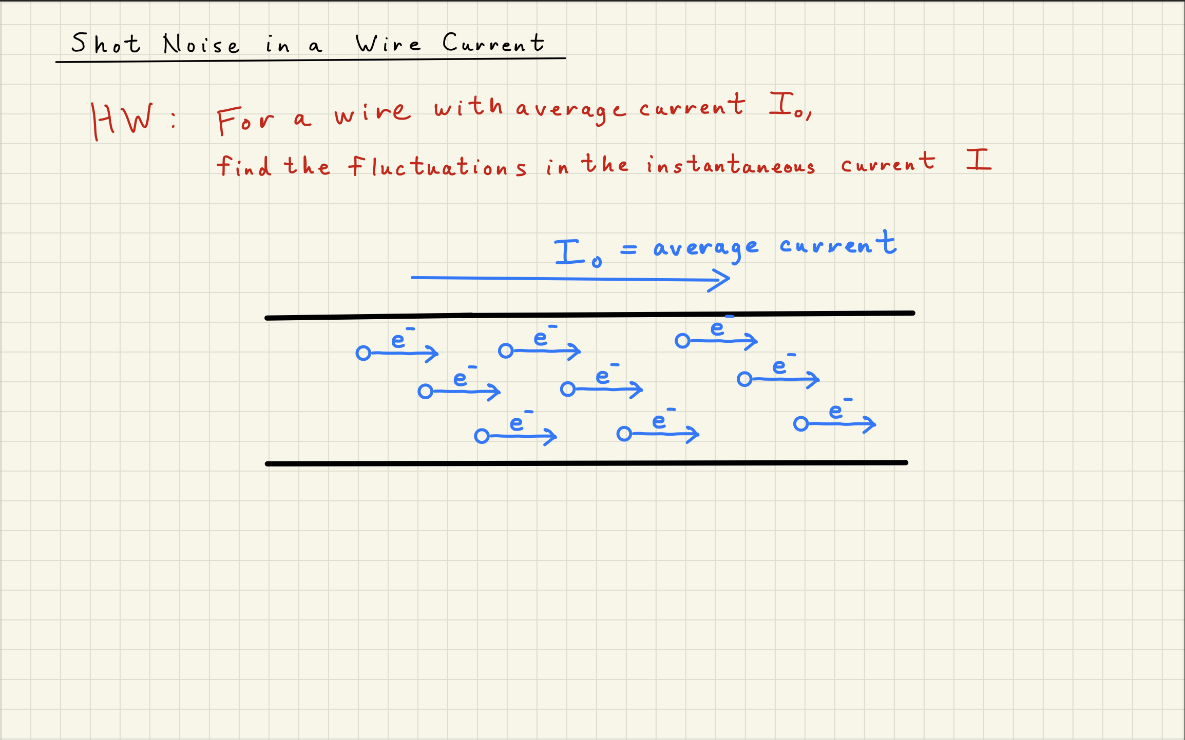
Shot noise is a limiting noise in gravitational wave detection and general detection.
Here are some things you may have heard about shot noise:
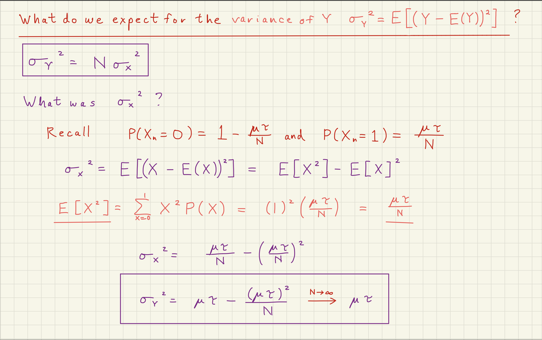
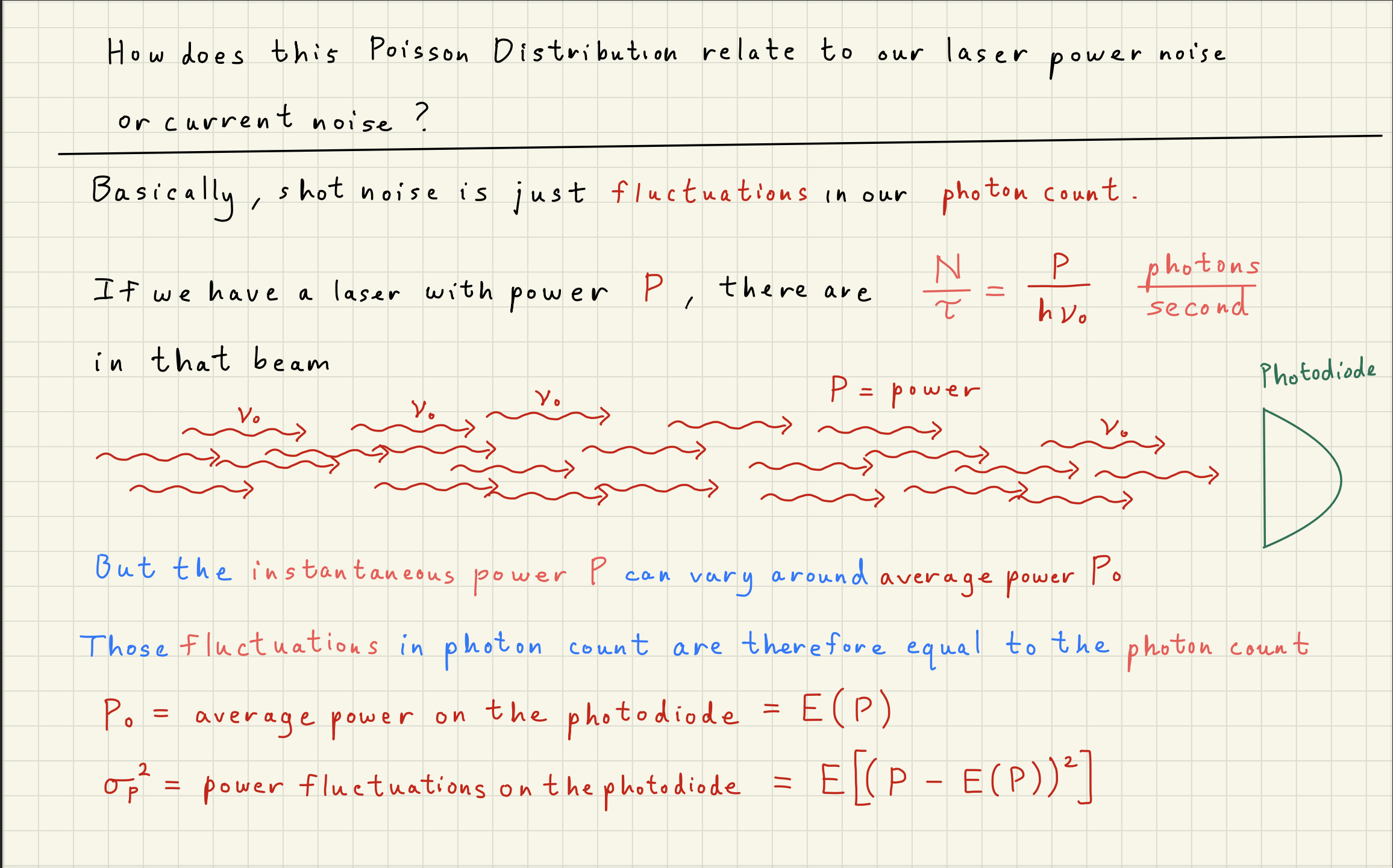
Shot noise is a quantum noise
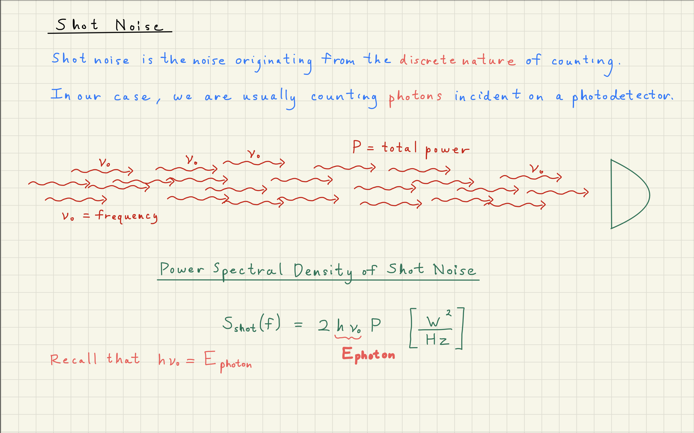
Shot noise comes from counting statistics
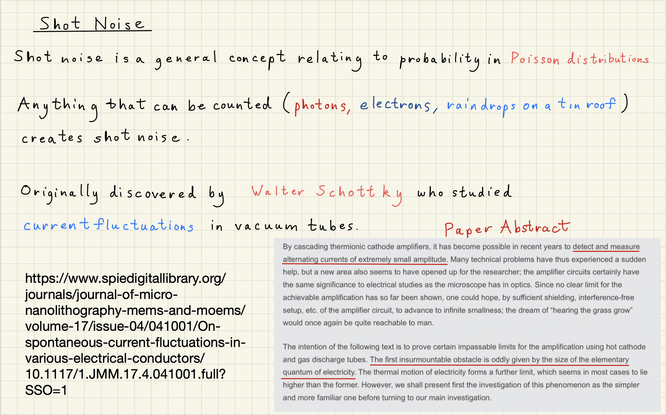
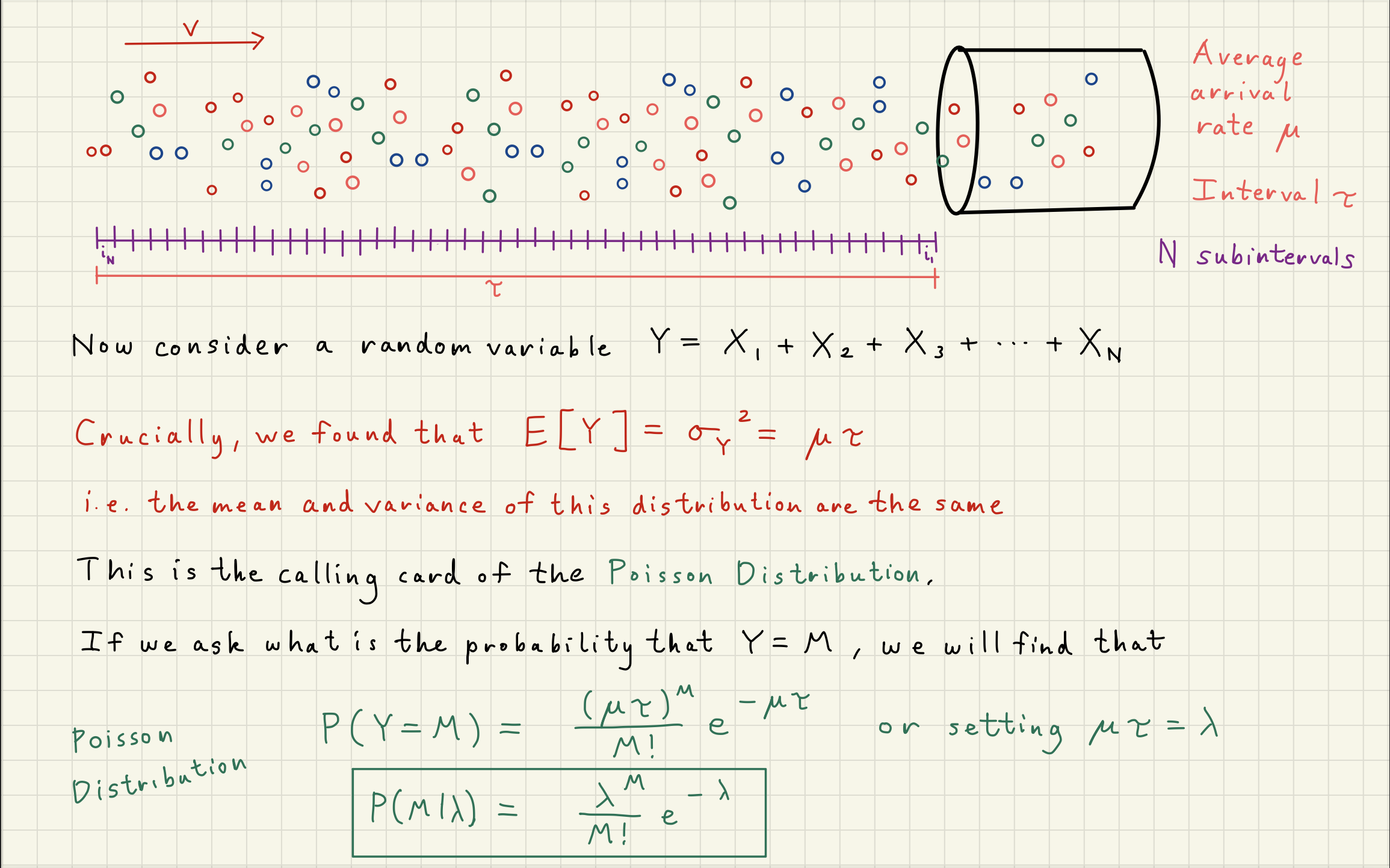
Shot noise is Poisson-distributed noise
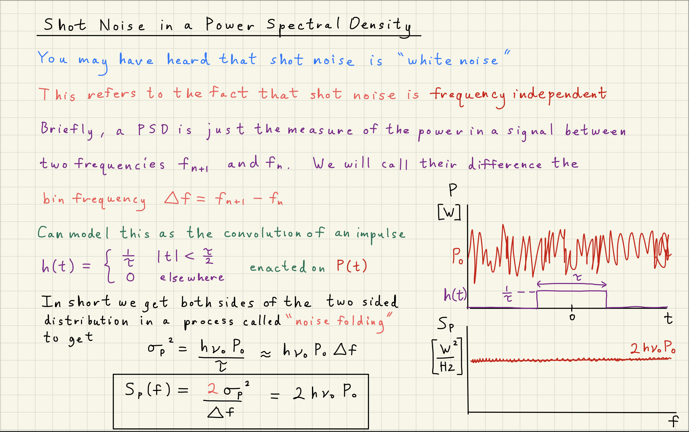
Shot noise is a white, Gaussian-distributed noise
Shot noise originates from Heisenberg uncertainty
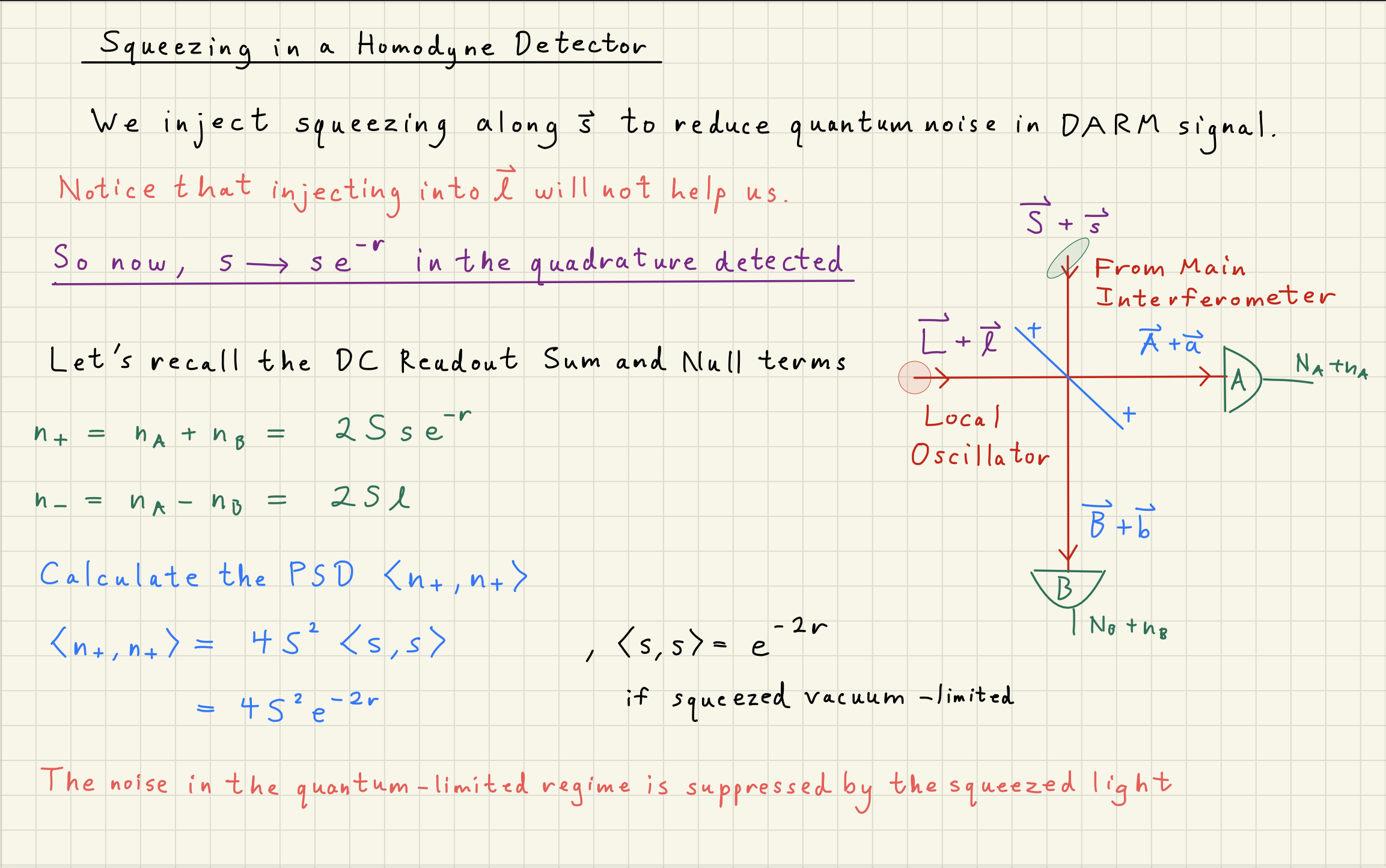
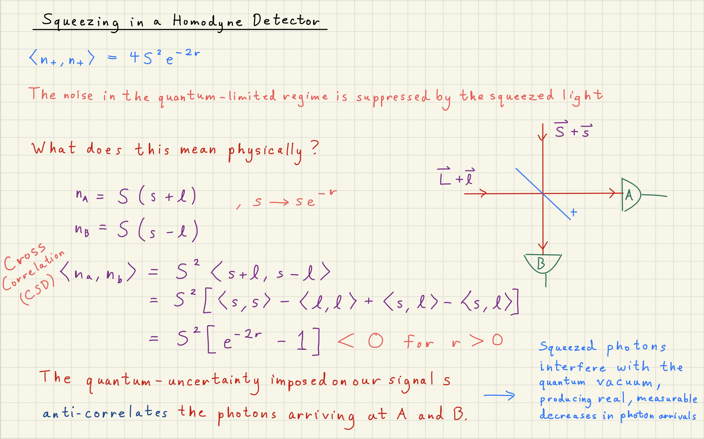
Shot noise can be squeezed by correlating photons
How does this entire picture hang together?
How can ``squeezing’’ the phase-quadrature of photons change their counting statistics?
Today, we’ll explore this picture and derive from first principles general shot noise.
Source
%matplotlib widget
import numpy as np
import matplotlib as mpl
import matplotlib.pyplot as plt
import scipy.signal as sig
import scipy.constants as scc
import matplotlib.gridspec as gridspec
from scipy.stats import poisson
from ipywidgets import interact, FloatSlider
from ipywidgets import *

plt.style.use('dark_background')

fontsize = 14
mpl.rcParams.update(
    {
        "text.usetex": False,
        "figure.figsize": (9, 6),
        # "figure.autolayout": True,
        # "font.family": "serif",
        # "font.serif": "georgia",
        # 'mathtext.fontset': 'cm',
        "lines.linewidth": 1.5,
        "font.size": fontsize,
        "xtick.labelsize": fontsize,
        "ytick.labelsize": fontsize,
        "legend.fancybox": True,
        "legend.fontsize": fontsize,
        "legend.framealpha": 0.7,
        "legend.handletextpad": 0.5,
        "legend.labelspacing": 0.2,
        "legend.loc": "best",
        "axes.edgecolor": "#b0b0b0",
        "grid.color": "#707070",  # grid color"
        "xtick.color": "#b0b0b0",
        "ytick.color": "#b0b0b0",
        "savefig.dpi": 80,
        "pdf.compression": 9,
    }
)1Shot Noise Derivation
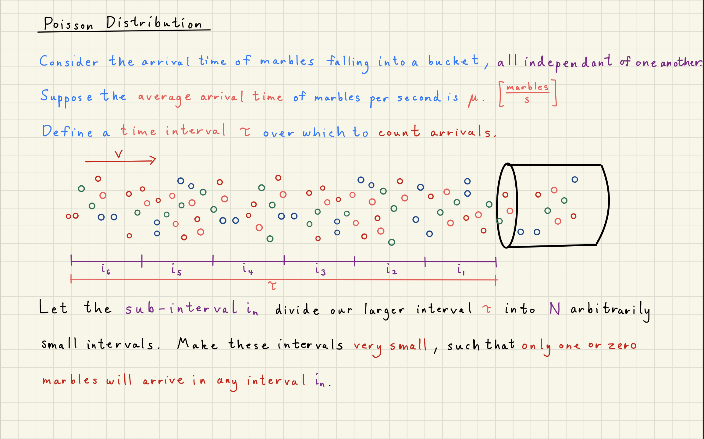
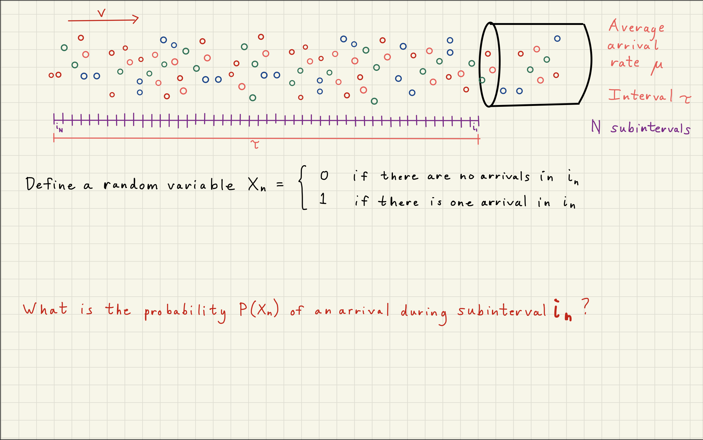
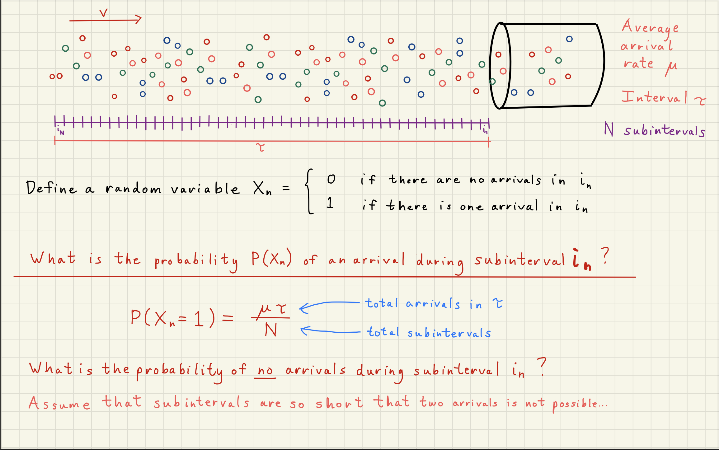
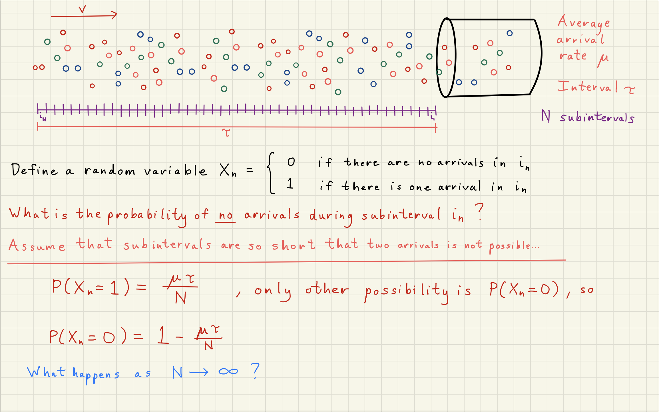
2Poisson Distribution Simulator
# Generate nn_samples of either 0 or 1
nn_samples = 100000
prob_0 = 0.9
prob_1 = 1 - prob_0

samples = np.random.choice([0, 1], size=nn_samples, p=[prob_0, prob_1])
nn_subset = 100
values_1 = np.sum(samples[:nn_subset])fig, ax = plt.subplots(figsize=(9, 3))
ax.stem(range(100), samples[:nn_subset], linefmt='C0-', markerfmt='C0o', basefmt='k-')
ax.set_xlabel("Sample index")
ax.set_ylabel("Value")
ax.set_title("First 100 binary samples, " + r"$N_1$" + f" = {values_1})")
ax.set_yticks([0, 1])
ax.set_ylim(-0.2, 1.3)
plt.tight_layout()
plt.show()n_chunks = nn_samples // nn_subset
# Reshape into (n_chunks, nn_subset) and sum each row to get count of 1s
chunks = samples[:n_chunks * nn_subset].reshape(n_chunks, nn_subset)
counts_of_1 = np.sum(chunks, axis=1) # number of 1s in each chunkfrom matplotlib.ticker import MaxNLocator
fig, ax = plt.subplots(figsize=(8, 5))
ax.plot(np.arange(len(counts_of_1)), counts_of_1, marker=".")
ax.axhline(prob_1 * nn_subset, color='C3', linestyle='--', linewidth=1.5,
label=f'Expected mean = {prob_1 * nn_subset:.0f}')
ax.set_ylabel("Number of 1s per chunk")
ax.set_xlabel("Chunk number")
ax.set_title(f"Plot of 1s across {n_chunks} chunks of {nn_subset} samples")
ax.legend()
ax.yaxis.set_major_locator(MaxNLocator(integer=True))
ax.grid()
ax.grid(which="minor", ls="--", alpha=0.3)
plt.tight_layout()
plt.show()x_bins = range(0,50)
# --- expected mean vline ---
mu = prob_1 * nn_subset
# --- Poisson overlay ---
# PMF scaled by n_chunks puts it in the same units as the histogram counts
pmf = poisson.pmf(x_bins[:-1], mu) * n_chunksfig, ax = plt.subplots(figsize=(8, 5))
ax.hist(counts_of_1, bins=x_bins, align='left',
color='C0', edgecolor='white', alpha=0.85)
ax.plot(x_bins[:-1], pmf, color='C1', label=rf'Poisson ($\mu$ = {mu:.1f})')
ax.axvline(prob_1 * nn_subset, color='C3', linestyle='--', linewidth=1.5,
label=f'Expected mean = {prob_1 * nn_subset:.0f}')
ax.set_xlabel("Number of 1s per chunk")
ax.set_ylabel("Count of chunks")
ax.set_title(f"Histogram of 1s across {n_chunks} chunks of {nn_subset} samples")
ax.legend()
plt.tight_layout()
plt.show()nn_samples = 100000
nn_subset = 100
n_chunks = nn_samples // nn_subset
x_bins = np.arange(nn_subset + 1)
fig = plt.figure(figsize=(9, 7))
gs = gridspec.GridSpec(2, 1, hspace=0.45)
ax1 = fig.add_subplot(gs[0])
ax2 = fig.add_subplot(gs[1])
# ── stem plot (top) ──────────────────────────────────────────────────────────
stem_container = ax1.stem(
range(nn_subset), np.zeros(nn_subset),
linefmt='C0-', markerfmt='C0o', basefmt='k-'
)
ax1.set_xlabel('Sample index')
ax1.set_ylabel('Value')
ax1.set_yticks([0, 1])
ax1.set_ylim(-0.2, 1.3)
# ── histogram + overlays (bottom) ────────────────────────────────────────────
bar_container = ax2.bar(
x_bins[:-1], np.zeros(nn_subset),
color='C0', edgecolor='white', alpha=0.75, label='Sampled chunks'
)
vline, = ax2.plot([], [], color='C3', linestyle='--', linewidth=1.5)
poisson_line, = ax2.plot([], [], color='C1', linewidth=2.0)
ax2.set_xlabel('Number of 1s per chunk')
ax2.set_ylabel('Count of chunks')
ax2.set_title(f'Histogram of 1s across {n_chunks} chunks of {nn_subset} samples')
def update(prob_1=0.30):
prob_0 = 1 - prob_1
samples = np.random.choice([0, 1], size=nn_samples, p=[prob_0, prob_1])
# --- top plot ---
first100 = samples[:nn_subset]
values_1 = int(np.sum(first100))
stem_container.markerline.set_ydata(first100)
stem_container.stemlines.set_segments(
[[[i, 0], [i, v]] for i, v in enumerate(first100)]
)
ax1.set_title(
f'First {nn_subset} binary samples, '
r'$N_1$' + f' = {values_1}, P(1) = {prob_1:.2f}'
)
# --- histogram ---
chunks = samples[:n_chunks * nn_subset].reshape(n_chunks, nn_subset)
counts_of_1 = np.sum(chunks, axis=1)
hist_vals, _ = np.histogram(counts_of_1, bins=x_bins)
for bar, h in zip(bar_container.patches, hist_vals):
bar.set_height(h)
# --- expected mean vline ---
mu = prob_1 * nn_subset
vline.set_data([mu, mu], [0, hist_vals.max() * 1.15])
vline.set_label(f'Expected mean = {mu:.1f}')
# --- Poisson overlay ---
# PMF scaled by n_chunks puts it in the same units as the histogram counts
pmf = poisson.pmf(x_bins[:-1], mu) * n_chunks
poisson_line.set_data(x_bins[:-1], pmf)
poisson_line.set_label(rf'Poisson ($\mu$ = {mu:.1f})')
ax2.relim()
ax2.autoscale_view()
ax2.legend()
fig.canvas.draw_idle()
slider = FloatSlider(
value=0.30, min=0.0, max=1.0, step=0.01,
description='P(1)',
continuous_update=True,
style={'description_width': 'initial'},
layout={'width': '500px'}
)
interact(update, prob_1=slider)
plt.show()In the above simulation, for a high probabilty of a 1 (beyond about 50%), the assumptions required for a Poisson distribution break down.
The concept of a zero and one flip, and zeros would become the “rare” result beyond 50%.
Additionally, a Poisson distribution becomes a Gaussian distribution for high mean values.
The spread of the Poisson distribution represents the variance, or noise, in our counting measurement.
This is what we call shot noise.
3White noise simulation
Now that we understand that the Poisson distribution is the underlying distribution describing shot noise, we can simulate the noise expected from any DC power signal.
For the below we’ll assume and
P_dc = 1e-3 # W
lambda0 = 1064e-9 # m
nu0 = scc.c / lambda0 # Hz
E0 = scc.h * nu0 # J, energy per photon
number_of_photons = P_dc / E0

# Estimate shot noise density in W^2/Hz directly from our equation
shot_noise_power_density = 2 * E0 * P_dc # W^2/Hz
shot_noise_amp_density = np.sqrt(shot_noise_power_density)

print()
print(f"DC power = {P_dc*1e3:.0f} mW")
print(f"number_of_photons = {number_of_photons:.3e}")
print(f"shot_noise_power_density = {shot_noise_power_density:.3e} W^2/Hz")
print(f"shot_noise_amp_density = {shot_noise_amp_density:.3e} W/rtHz")
DC power = 1 mW
number_of_photons = 5.356e+15
shot_noise_power_density = 3.734e-22 W^2/Hz
shot_noise_amp_density = 1.932e-11 W/rtHz
##############################################
#   Simulate a our time domain signal P(t)   #
##############################################
# To simulate P(t), we need a sampling frequency fs to see what our noise power will be.
# Set up the FFT

avg = 10                         # number of averages
fs = 1e4                         # Hz, sampling frequency, samples/second
NN = (avg + 1) * 1000            # number of samples
total_time = NN / fs             # seconds, total time

nperseg = 1000                  # number of samples in a single fft segment
noverlap = 0 #nperseg // 2      # 0% overlap

bandwidth = fs / nperseg
overlap = noverlap / nperseg

averages = (total_time * bandwidth - 1)/(1 - overlap) + 1

print()
print(f'total samples NN = {NN}')
print(f'sampling frequency = {fs} Hz')
print()
print(f'total_time = {total_time} seconds')
print(f'bandwidth = {bandwidth} Hz')
print(f'overlap = {100 * overlap} %')
print(f'averages = {averages}')
total samples NN = 11000
sampling frequency = 10000.0 Hz

total_time = 1.1 seconds
bandwidth = 10.0 Hz
overlap = 0.0 %
averages = 11.0
# We can only capture signals up to the Nyquist frequency = fs/2,
# so our total noise power is = noise density * Nyquist frequency
shot_noise_power = shot_noise_power_density * fs / 2    # total power in the noise spectrum in W**2.
                                                        # Equal to the variance of the gaussian noise.
# Simulate the power time domain signal P(t)
# We want NN samples with a variance = shot_noise_power, or a standard deviation of sqrt(variance)
power_t = np.random.normal(loc=P_dc, scale=np.sqrt(shot_noise_power), size=NN) # sqrt(noise_power) = sigma on guassian noise# Take the spectral density
ff, Sxx = sig.welch(power_t, fs, nperseg=nperseg, noverlap=noverlap)
Axx = np.sqrt(Sxx)fig, ax = plt.subplots(figsize=(8, 5))
ax.plot(power_t[:200])
ax.axhline(P_dc, color='C3', linestyle='--', linewidth=1.5,
label=f'Mean Power = {P_dc*1e3:.0f} mW')
ax.set_ylabel("Power P(t) [W]")
ax.set_xlabel("Sample Number")
ax.set_title(f"Power Measurement P(t)")
ax.legend()
# ax.yaxis.set_major_locator(MaxNLocator(integer=True))
ax.grid()
ax.grid(which="minor", ls="--", alpha=0.3)
plt.tight_layout()
plt.show()fig, ax = plt.subplots(figsize=(11, 5))
ax.loglog(ff, Axx, label="Measured Power ASD")
ax.axhline(shot_noise_amp_density, color='C3', linestyle='--', linewidth=1.5,
label=f'Shot noise = {shot_noise_amp_density:.2e} W/rtHz')
ax.set_ylim([1e-11, 1e-10])
ax.set_ylabel("Power ASD "+r"$[\mathrm{W/\sqrt{Hz}}]$")
ax.set_xlabel("Frequency [Hz]")
ax.set_title(f"Power ASD " + r"$\sqrt{S_{PP}}$")
ax.legend()
# ax.yaxis.set_major_locator(MaxNLocator(integer=True))
ax.grid()
ax.grid(which="minor", ls="--", alpha=0.3)
# plt.tight_layout()
plt.show()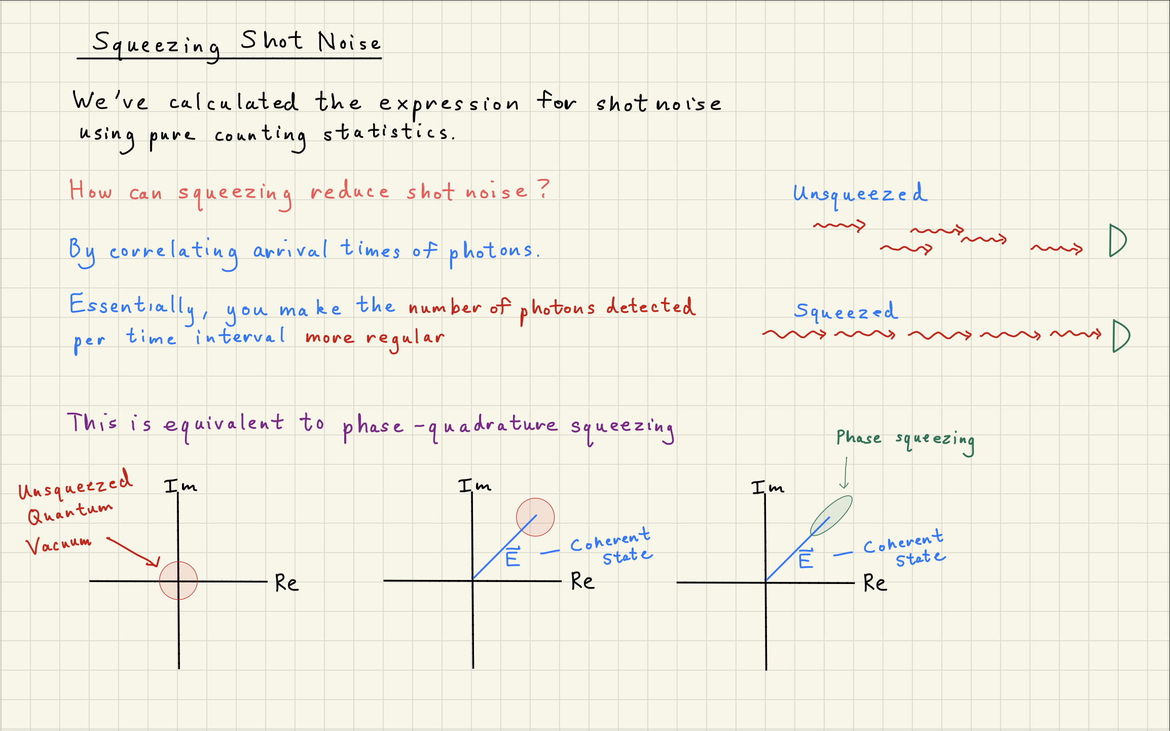
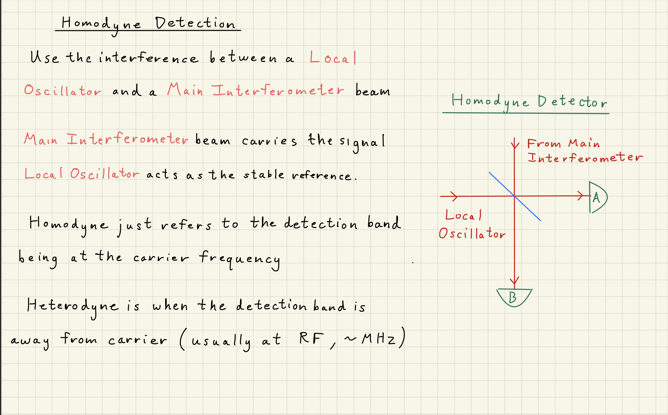
4Homodyne Detector